Introduction
The capital assets prices model was developed to illustrate the way prices of a risk is informed by the influence of investors’ preferences and the physical characteristics of the capital assets (Easton, 2009). It shows the relationship between an asset’s price and the risks associated with it. At the time of its development, economist lacked enough microeconomic theory to explain the conditions of risks in the capital market (Sharpe, 1964). Consequently, it was difficult to link the price of a given asset and the risk associated with it. This paper will analyze the concept of capital asset prices. The main contributions and limitations of the model will be illuminated.
Investors’ Preference Function
To begin with, let us consider the assumption that the results of an investment is in the form of a probability distribution. In an attempt to evaluate the suitability of a given investment, the investor can consider two parameters namely, the expected value of the investment and the standard deviation associated with it (Sharpe, 1964). The preference of the investor can thus be “expressed in terms of the total utility function” (Sharpe, 1964) which is illustrated as follows:
U= f(Ew, δw) where, Ew is “the expected amount of wealth in future and δw is the predicted standard deviation” (Sharpe, 1964) which shows the extent to which the future wealth will diverge from Ew.
This model is based on the assumption that investors “prefer a higher expected future wealth to a lower value, ceteris paribus” (Sharpe, 1964). This means that dU/dEw will be greater than zero. The model is also based on the assumption that investors are risk-averse (Sharpe, 1964). Thus they will opt for an investment associated with a smaller value of δw instead of another investment associated with a greater value of δw when dU/ dδw < 0 (Bruetsch, 2009). These assumptions mean that the indifference curve showing the relationship between Ew and δw will be slopping upwards. Thus if an investor decides to invest a portion of his or her present wealth, W1, the rate of return on the investment can be given as:
R= (Wt – W1)/ W1 and Wt = RW1 + W1 where, Wt is the expected future wealth and R is the investment’s rate of return. The investor’s preference can thus be expressed as U=g(ER, δR). This function is based on the fact that terminal wealth has a direct relationship with the rate of return (Choudhry, 2002).
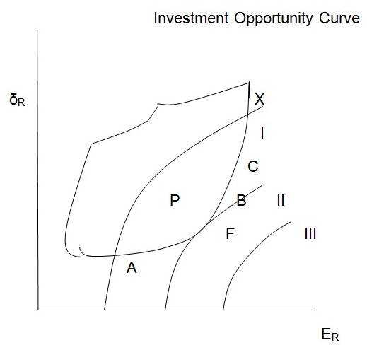
In the above figure, it is assumed that the investor is rational and thus given a set of investment opportunities, he or she will opt for the opportunity associated with maximum utility (Sharpe, 1964). The graph of ER and δR , represents all the investment options available to the investor. If all these investment options are associated with some risk, then the area marked P will represent the investment options. Since the investor intends to maximize returns, he or she will choose an investment option that “places him on the indifference curve associated with the highest level of utility” (Sharpe, 1964). The investor can choose such an investment option in the following way. The first step involves identifying the most efficient combination of available investment options (Koller & Goedhart, 2010). At the second stage, the investor will pick one option from the combinations identified in step one. An investment plan or option will be considered efficient if and only if the following conditions apply. First, there is no an alternative plan with an equal ER and a lower δR. Second, there is no an alternative option with the same level of δR and a greater ER. Third, there is no an alternative option associated with a greater ER and a lower δR. Therefore, in the above figure only points on the “lower right-hand of the curve AFBDCX” (Sharpe, 1964)will be chosen.
Assuming two investment plans A and B, the process of choosing the most efficient plan can be illustrated mathematically as follows. By investing part of the investor’s wealth, α, in A and the rest (1- α) in B, the rate of return expected form this combination can be given as follows:
ERc = αERa + (1-α)ERb
The forecasted standard deviation associated with the combination can be given as:
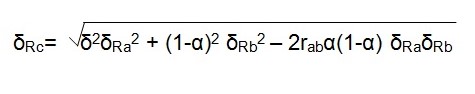
from the above formula, a positive value means that the investor associates the outcome of the two investment options with a positive relationship (Sharpe, 1964). A zero value implies that the results of the two investment options are indifferent. A negative value on the other hand implies an inverse relationship between the outcomes of the two investment options (Focardi & Fabozzi, 2004).
The Pure Risk of Interest
Assuming P is a riskless asset (δRp=0) and its expected rate of return is equivalent to the pure interest rate. If part of an investor’s wealth, α, is invested in P and the rest invested in a risky asset A, the expected rate of return will be ERc =αERp + (1-α) ERa. The standard deviation associated with this combination can thus be given as:
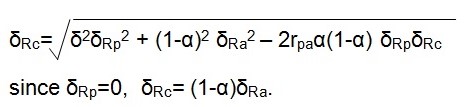
This means that all combinations of investment options involving some “risky asset, δRc, must have values of EFc and δRc which lie along a straight line between the points representing the two components” (Sharpe, 1964).
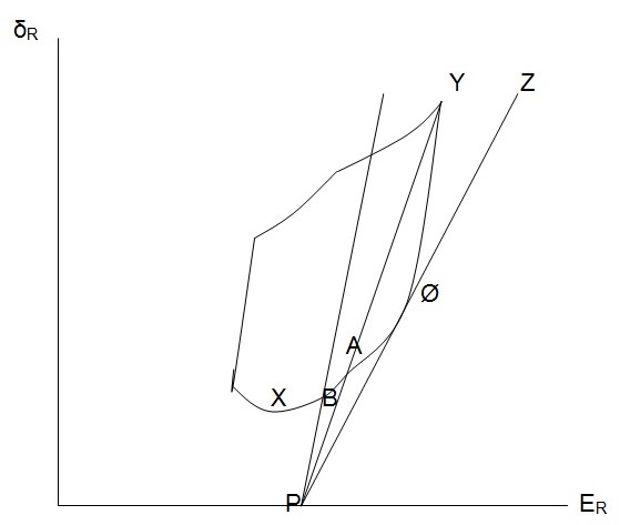
In the figure above, the combinations of ER and δR on the line PA can be attained if some amount of money is loaned at the pure interest rate and part of it is invested in A (Koller & Goedhart, 2010). In a similar way, if at the pure interest rate some amount of money is lent and invested in B the combinations existing on line PB can be attained. In all the cases, one investment option will dominate. The dominant investment plan will be the one found at the “original investment opportunity curve where a ray from point P is tangent to the curve” (Sharpe, 1964).
In the case of borrowing, an investor’s ability to borrow at the pure interest rate is the same as divesting in P (Fabozzi & Drake, 2009). By letting α assume negative values in the equations obtained in the case of lending, it will be possible to determine the consequences of borrowing with the aim of acquiring a given investment in excess of the amount that can be purchased with the existing amount of wealth. This is represented by the points on the extension of line PA in the event that the borrowed money is used to purchase A. If the borrowed money is used to purchase B, the effect will be represented by the points on the extended PB line. It is worth noting that a given investment plan will dominate the rest. When the lending and borrowing rates are equivalent, the dominate investment plan will be the same in the case of both lending and borrowing (Focardi & Fabozzi, 2004). Consequently, the investment opportunity curve will be transformed into a line (PøZ) (Sharpe, 1964). In the event that the original investment opportunity curve fails to be linear at ø, the efficient investment plan can be chosen as follows. The first step involves identifying the optimum combination of assets associated with some risks. The second stage involves borrowing or lending in order to identify the specific point on line PZ where an “indifference curve is tangent to the line” (Sharpe, 1964).
Equilibrium in the Capital Market
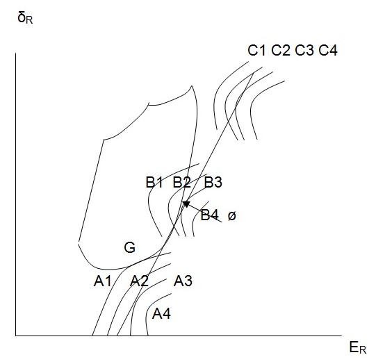
Determining the equilibrium in the capital market is based on two assumptions. First, a pure interest rate is assumed (Clark & Mountford, 2007). Besides, each and every investor is expected to be in a position to borrow or lend money at equal terms. Second, the expectations of investors are assumed to be homogenous. Based on these assumptions, when investors are faced with a set of capital asset prices, they will view their alternatives in a similar manner (Schwartz, Carew, & Tatiana, 2010). An investor whose preferences are indicated by the indifference curves labeled A1 to A4 in the figure below will be interested in lending a better portion of his money at the pure interest rate. Such an investor would invest the balance of his money in the investment or asset combinations represented by point ø. This is due to the fact that such a combination will enable him to attain the optimum point A* (Sharpe, 1964). An investor whose preferences are represented by the indifference curves labeled B1 to B4 will be interested in investing his money in combinations represented by ø. For an investor exhibiting the preferences represented by C1 to C2, it will be in his interest to invest all his money and any other additional funds at ø (Sharpe, 1964). This will enable him or her to reach the preferred point C*.
The process of purchasing asset combinations represented by ø while avoiding to purchase the assets not represented by combination ø, leads to revision of prices. The change in prices will lead to a change in investors’ actions. This means that the investors will find some combinations to be more attractive (Schwartz, Carew, & Tatiana, 2010). This results into different demand and further price revisions. The change in prices is expected to continue until the attainment of a price level at which all assets can “enter at least one combination lying on the capital market line” (Schwartz, Carew, & Tatiana, 2010)
Equilibrium point:
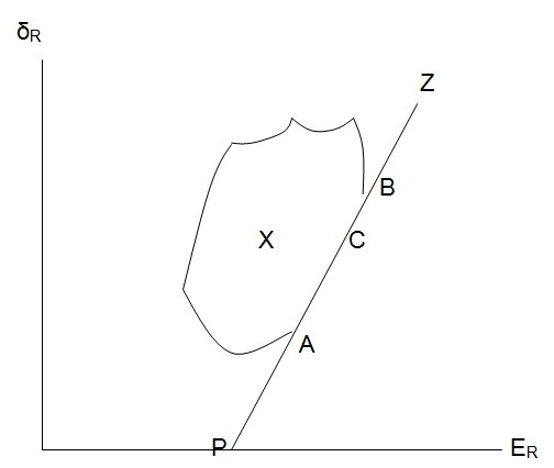
The possible combinations in the area marked X in the figure above can be attained by combining risky assets. Points on line PZ can be reached through “lending or borrowing at the pure interest rate plus an investment in some combination of risky assets” (Sharpe, 1964). Effective combinations can be obtained by combining various risky assets. Besides, such combinations should be positively correlated. This illustrates the relationship between asset’s price and the risks associated with it.
Prices of Capital Assets
The perfect correlation associated with effective combinations is attributed to the dependence on prevailing economic activity (McConnell & Brue, 2007). In such a case, investors will be able to avoid all risks except those attributed to economic surveys through diversification. Price adjustments will continue until a linear relationship linking the response to economic activity and the expected rate of return is attained (McConnell & Brue, 2007). The assets which are not affected by the changing economic activities yield the same returns (Sharpe, 1964). Assets which are affected by the changes in economic activity will yield a higher return.
Limitations
First, the model considers variance of returns to be an effective measure of risk (Sharpe, 1964). This assumption can only apply in the case of normally distributed returns (Boyes & Melvin, 2006). In the case of generally distributed returns, this measure will not be effective. This is because the risk associated with financial investment is not a variance but a probability of loosing. Second, the assumption that investors have homogenous expectations does not apply in all cases (Krugman & Wells, 2009). In reality investors do not have access to the same information about the market while investing. Besides, it is not easy to find all investors agreeing on the level of risk and the expected returns since they all have different expectations (Javid & Ahmad, 2005). Third, the model is based on the assumption that investors’ probability beliefs are equivalent to actual distribution of returns. However, in the actual sense the investors’ expectations may be biased (Gray, Hull, & Kleas, 2009). Fourth, the variance of stock returns is not properly addressed. This is because research indicates that stocks associated with lower beta values “generate greater returns than the model can predict” (Gray, Hull, & Kleas, 2009). Finally, in theoretical sense the market portfolio includes all types of assets. However, in practical sense it is not possible to observe such a market portfolio. Besides, investors normally “substitute stock index as an alternative for the true market portfolio” (Aikman & Paustian, 2006). However, the model undermines the significance of this substitution. Thus false inferences can be made using the model. These limitations undermines the effectiveness of the model as a tool for analyzing the capital market and prices of assets.
Conclusion
The capital asset price model was developed to provide a microeconomic foundation in the analysis of the capital market (Boyes & Melvin, 2006). Its main contribution was that it enabled the investors to link the prices of various assets to the risks associated with such assets. Diversification is used to reduce the level of risks involved in financial investment (Clark & Mountford, 2007). The model uses the variance of returns as the measure of risks (Sharpe, 1964). Despite its contributions in the field of financial investments, the model also has limitations. One the major limitation of the model is that variance of returns can not provide an effective measure of risks (Schwartz, Carew, & Tatiana, 2010). Besides, testing the model is challenged by the inability to observe the market portfolio as discussed above.
References
Aikman, D., & Paustian, M. (2006). Bank capital, asset prices and monetary policy. Theorectical and Applied Economics, 6(4) , 47-54.
Boyes, W., & Melvin, M. (2006). Economics. New York: Cengage Learning.
Bruetsch, M. (2009). From capital market effects to behavioral finance. New York: GRIN Verlag.
Choudhry, M. (2002). Capital Market instruments. New York: FT Press.
Clark, G., & Mountford, D. (2007). Investment strategies and financial tools for local development. Boston: OECD Publishing.
Easton, P. (2009). Estimating the cost of capital implied by market prices. Hanover: Now Publishers.
Fabozzi, F., & Drake, P. (2009). Finance: capital market, finacial management and investment. New York: John Wiley and Sons.
Focardi, S., & Fabozzi, F. (2004). The mathematics of financial modelling and investment management. New York: John Wiley and Sons.
Gray, S., Hull, J., & Kleas, D. (2009). Bias, stability and predictive ability in measurement of systematic risk. Accounting Research Journal, 22(3) , 220-236.
Javid, A., & Ahmad, E. (2005). The conditional capital asset pricing model: evidence from Karachi Stock Exchange. Theorectical and applied Economics, 4(2) , 24-36.
Koller, T., & Goedhart, M. (2010). Valuation. Boston: McKinsey & Company Inc.
Krugman, P., & Wells, R. (2009). Economics. Boston: Worth Publishers.
McConnell, C., & Brue, S. (2007). Economics. New York: McGraw-Hill.
Schwartz, R., Carew, M., & Tatiana, M. (2010). Micro Markets:a market structure approach to macroeconomic analysis. New York: John Wiley and Sons.
Sharpe, W. (1964). Capital asset prices: a theory of market equilibrium under conditions of risk. Journal of Finance, 19(2) , 425-442.