The Analysis of Efficient Portfolio

Introduction

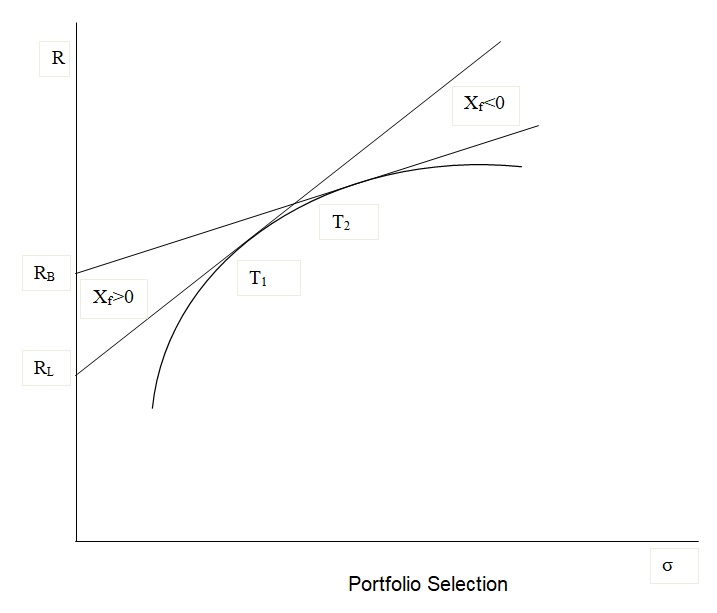
According to Luenberger (1997), the relationship between risk and return of risky assets in the market can be investigated by determining the effects of different borrowing and lending rates. This analysis is done by first constructing a portfolio that consists of only risky assets, which results in the determination of the minimum-variance portfolio. After this determination is completed, the efficient frontier is then determined, after which a risk-free asset is introduced in the portfolio. The introduction of a risk-free asset in the portfolio results in an efficient frontier that explains the effect of having different interest rates for borrowing and lending, as is depicted in the diagram below.

The portfolio selection problem is an issue that has been discussed for a long time by both theoretical and practical investors. Until the current period, different models of portfolio selection have been developed and researched for studies and investment in the portfolio market, though the research results in previous periods were based on a simple version of the complex financial markets. An example of this fact is that the earliest market variance model assumed that the financial markets were operated in a frictionless economy that had a discrete-time distribution, allowed for boundaryless short-selling of assets, and had no risk-free assets. This early model was modified to give the revised Markowitz’s model that allowed risk-free operations in the market and allowed the practice of short-selling. This model can now be modified to include different rates for borrowing and lending, a fact that is studied in this paper to decide the optimal portfolio choice in a market that allows for different rates for borrowing and lending and allows limitless short-selling of assets. The allowance of different rates for borrowing and lending in the market means that an investor gets the chance to perform margin transactions if desired; that is the investor is allowed to borrow as a means of financial leverage (Copeland and Weston, 2004).

According to Lintner (1965), the rationale for the allowance of different rates for borrowing and lending is explained by the fact that, in the market, there has to be effective market capitalization. This is because a lack of efficiency in the market would give all investors the justification to borrow and lend at the same rate, which would lead to insufficient market capitalization. This inefficiency is explained by the lack of sufficient information and theories of efficient market hypothesis, which explain the way a lack of information affects market operation. The theories of information in the market explain that investors in any market are imperfectly informed about the market, meaning that lenders do not understand the behaviors of borrowers in the market. For example, some borrowers like the government have reputations of perfect credit histories, while private investors cannot guarantee the same credit rating (Elton et al, 2002). Therefore, the investors who have good credit ratings can borrow at low-interest rates, while private investors with unknown credit ratings borrow at higher interest rates. Another fact that explains the differences in borrowing and lending rates is the fact that lenders do not usually have as much information as borrowers, which results in the borrowers having to pay extra interest on their debts. This disparity exists so that lenders can compensate for the lack of sufficient information on market demographics, which leads to increased risk on the investments that they make. The main effects of the difference in borrowing and lending rates are that the efficient portfolio cannot be defined by a straight tangent, and investors will face an efficient frontier that is determined by the rates at which they can borrow (Arrow, 1971).

In the above diagram, the portfolio is constructed with the assumptions that the expected return for the risky asset is bigger than the expected return for the risk-free asset, the rates for borrowing are greater than the lending rates, and the expected pay off from the portfolio is determined by the expected payoffs of the risky assets. The explanation of the above graph will start with a description of the efficient frontier, how it is derived, and the assets and conditions that make up the efficient frontier. To investigate this, this paper will focus on the introduction of two risky assets in a market where short-selling is not allowed, and the relation between risk and return of the assets is called the portfolio frontier, whose shape can be determined to depend primarily upon the coefficient of returns among the returns of the two assets. After this analysis, short-selling is allowed so that the portfolio has a practical implication, a factor that will be seen to expand the frontier but retain its shape.

Efficient Portfolio Theory

Consider a market where there are two risky assets, A and B, whose expected returns are assumed to be different, ne short-selling is allowed, and there is no risk-free asset. The analysis of his portfolio will begin by assuming that the return for the two assets are defined by the relationship r_a < r_b, which means that for any investor to decide to invest in asset A, the asset must have a lower variance than asset B, σ_A² < σ_B². This implies that if these conditions are ignored, both assets would be ignored, or there would be no problem with choice because the return and variance would be the same (Jacques, 1999).

An investor makes a portfolio which has two risky assets by considering that the two assets have proportional holdings in the portfolio, and if short-selling is not allowed, it means that the holdings of both assets must be positive. This is analyzed by focusing on the relationship between the standard deviation and the expected return of the whole portfolio, an analysis that will reveal the way in which investment can be done to substitute the risk of a portfolio with its return.

According to Chiang (1984), from the mean variance formula, the risk or standard deviation of a two-asset portfolio is determined to be from the following computation:

If the variances of the two assets are then considered, it means that the risk of the portfolio will depend solely on the value of the correlation coefficient of the data set, ρ_AB. When two assets are considered, there are two choices for the correlation coefficient, either the correlation is perfectly positive, +1, or the correlation is perfectly negative, -1. In the case where the correlation coefficient is perfectly positive, it can be determined that the expected return is always a weighted sum of the expected earnings of the individual assets, while in the case of the negatively correlated assets, it is determined that the expected return is a weighted sum of the return of the assets with one of them being negative. The graph displayed above shows the efficient frontier as a straight line, and this is determined from the equation of the portfolio of two risky assets whose expected return is a weighted average of the expected returns of the two assets. Therefore, from the efficient frontier derived, it is evident that the investor can substitute the accompanying risk of a portfolio with the return earned from the portfolio, which gives the frontier the name, portfolio frontier. According to Roll (1977), the efficient frontier displays that there is no portfolio which has a null standard deviation; therefore, the portfolio is termed a minimum-variance portfolio, since the investor aims to minimize the associated risk in a portfolio containing risky assets.

The efficient portfolio frontier can be generalized to include all other risky assets by introducing the notion of short-selling and risky assets. As already summarized, the efficient portfolio for any investor is the set of points that contain the assets with the least variance and the maximum return, so for many portfolios, an investor can create an efficient frontier by investing only in the assets mentioned above.

The introduction of short-selling into a portfolio would change the investment proportions in the two assets A and B, since short-selling technically means the selling of an asset if the price drops and reinvesting the return in the other risky asset. With the introduction of short-selling, an investor would ne able to make an infinite return from two risky assets in a portfolio because the reinvestment would not stop at the sale of one asset. With the issue of short-selling, the efficient frontier would change because the upper boundary of the investment in one risky asset would not change to infinity because of the reinvestment in the asset. For example, with two risky assets, A and b, an allowance of short-selling of one asset expected return of A is higher than the expected return for A would mean that the continuous short-selling of B is done. The return from the short-selling of B would then be invested in the risky asset A, therefore, ensuring that there is an infinite positive return on the asset A (Elton et al, 2002).

Generalization to Capital Market Equilibrium

The portfolio choice defined in the preceding section can then be generalized to a capital market equilibrium that describes the expected return to any asset by defining the portfolio to become an optimal risky portfolio. As already stated, an investor will always aim to minimize the standard deviation (risk) of a portfolio (Pratt, 1964). The discussion already done introduced the notion of the minimum-variance portfolio, which stated that the expected return and the variance of a portfolio was equal to the weighted sums of the relevant aspects of the each asset. However, to get the optimal risky portfolio, the minimum-variance portfolio is equated to a predetermined expected rate of return, which essentially means that the investor requires the portfolio to behave in a particular manner. The formula for this is:

,

Subject to the condition that

, where the investor expects a return equal to E^* and that the weights of the assets invested must be equal to a sum of 1;

To solve this equation, the function can be equated to a Langrarian system to get the constraint equation,

which can be solved by partially differentiating the equation with respect to each of the variables present in it. After the differentiation is done, the resultant equation is solved algebraically to give the investor the optimal return portfolio. However, if the short-selling constraint is disallowed, the constraint that dictated that the weights of the portfolios must equal to one will have to be modified to become

, which means that the absolute values of the portfolios must be equal to one. This will eliminate the chance of a nonnegative portfolio failing to make it into the asset list, which would mean the elimination of one asset (Merton, 1972).

According to Miller (1975), after the optimal portfolio has been obtained, the next task is the allocation of the optimal risky portfolio, which is the primary reason why an investor would want to generalize the model into a capital market equilibrium model. The decision by an investor to take on the risk of a portfolio is affected by the amount of risk aversion that the investor has, meaning the rate at which an investor is willing to substitute the risk of a portfolio with the expected return, this level of risk can be determined by finding the level of indifference that the investor has to risk, which is done by determining the investor’s indifference curve that reflects the coinciding levels of risk and return (.

The indifference curve determines the amount of risk that an investor is willing to take on before a substantial level of return is arrived at in the portfolio. To determine this factor for each investor, the analyst will use the utility function for each investor, which is a reflection of the average satisfaction that the investor will achieve with the investment in the risky assets. The utility function is simply a risk/return trade-off matrix for the investor and assigns a portfolio to a given level of return and risk. The utility function is described as:

, where U is the amount of utility derived from the investment, A is the amount of the risk aversion, the constant is a value that allows the analyst to express the risk and return in terms of numerical percentages, and the standard deviation is measured by sigma. The risk aversion figure will change from a low value of 0 to a high value as the investor goes higher in the risk aversion scale (Merton, 1972).

Therefore, to determine the portfolio for every investor, the independent utility functions for the investor are plotted in the same graph with the efficient frontier curves for all the investments that are available for the investor to make, where an investor is less risk averse if the utility function is lower than all the other investors. From the plot of the curves, the deduction is made that an investor will pick the optimal portfolio where the curve produces the highest utility for the level of indifference to risk, which is the point where the utility curve and the efficient frontier are at a tangent. From this analysis, it is evident that every investor will pick the point that maximizes the return from the portfolio and minimizes the standard deviation or variance (Merton, 1972).

According to Statman (1987), for an investor to find a simpler way of finding the optimal portfolio balance, a new curve called the CAL is introduced, which shows all the possible combinations of earnings and standard deviations of the portfolio and allows the investor to choose the one that is most appealing. The capital allocation line is used by the investor to determine the capital market equilibrium that defines the expected return to market of any risky asset in the portfolio. To derive the capital allocation line, the first step is the determination of the weights of the two risky assets which will give the highest result for the CAL, therefore, maximizing the return that is earned on the investment (Sharpe, 1964). If the objective function is defined as CAL_s, the equation with the weights of the risky assets, W_A and W_B, is given as:

, and the expected return and associated standard deviation are given as

and

respectively. The maximization of the equation containing

subject to the constraint

is

, which, when solved, gives the solutions of the weights of the two assets as:

According to Black (1972), the optimal risky portfolio can be formed for the capital equilibrium by considering the above equation in the view of the risk-averse investor by combining the capital allocation line, the risk-free asset and the risky assets in the portfolio. Finally, taking the assumption that the risk-free asset is represented by r_f, and the return of the portfolio as E (r_P), the earnings of the final portfolio is given as

, and the variance is defined as 

. Therefore, the solution for the portfolio choice problem when it is generalized to a capital market equilibrium that describes the expected return to any assets in the market is given by the model derived above (Greene, 2000).

References

Arrow, J. (1971). Essays in the Theory of Risk Bearing. Stamford: Markham Publishing Company.

Black, F. (1972). Capital Market Equilibrium with Restricted Borrowing. Journal of Business. Vol. 45, Pp. 444-455.

Chiang, C. (1984). Fundamental Methods of Mathematical Economics. New York: McGraw-Hill.

Copeland, E., and Weston, F. (2004). Financial Theory and Corporate Policy. Boston: Addison-Wesley.

Elton, J., et al. (2002). Modern Portfolio Theory and Investment Analysis. New York: John Wiley and Sons.

Greene, W.H. (2000). Econometric Analysis. London: Prentice Hall.

Jaques, I. (1999). Mathematics for Economics and Business. Boston: Addison-Wesley

Lintner, J. (1965). The Valuation of Risk Assets and the Selection of Risky Investments in Stock Portfolios and Capital Budgets. Review of Economics and Statistics. Vol. 47. Pp.13-37.

Luenberger, D. (1997). Investment Science. London: Oxford University Press.

Merton, R.C. (1972). An Analytic Derivation of the Efficient Portfolio Frontier. Journal of Financial and Quantitative Analysis. Vol. 7. Pp. 1851-1873.

Miller, S.M. (1975). Measures of Risk Aversion: Some Clarifying Comments. Journal of Financial and Quantitative Analysis. Pp. 299-309.

Pratt, J.W. (1964). Risk-Aversion in the Small and in the Large. Econometrica. Vol. 32 Pp. 122-136.

Roll, R. (1977). A Critique of the Asset Pricing Theory’s Tests, Part I. Journal of Financial Economics. Vol. 4. Pp. 129-176.

Sharpe, W.F. (1964). Capital Asset Prices: A Theory of Market Equilibrium under Conditions of Risk. Journal of Finance. Vol. 19. Pp. 425-442.

Statman, M. (1987). How Many Stocks Make a Diversified Portfolio? Journal of Financial and Quantitative Analysis. Vol. 22. Pp. 353-363.