The best way to use while using this method in a time series model is through generalizing differences between the two sets of data. If the standard deviation if the data is unknown the following equation is used.
Yt =ztβ + ut
Yt-1 =xt -1β + ut -1 multiply by σ and subtract it from the above line to get;
Yt –yσt-1 =xtβ –σxt-1β +ut –σut -1
Where:
- t is time
- σ is the standard error

Once the data has been incorporated together by generalizing the differences using the first linear explanation the second linear expression is obtained through this residues are estimated which are then regressed together without any interception since the mean is = o after passing through this processes autocorrelation is removed.
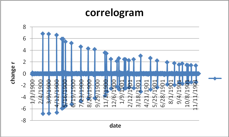
The correlogram shows that the data is randomly distributed. It does not follow any criteria. Historical data is adjusted to reflect the current estimation in the market. A mean is the average of the data set. A mean is calculated for discrete and no discrete data. A mean is important in determining the values of returns of data. It is at times considered to be a return (Gracas, Colares and Sandre-Pereira 2001).
A variance is a standard error of a data set and is calculated using the standard errors from the mean of all the data set. Then the standard error of the total data is obtained. It can be simply described as time-series data standard errors which are calculated as shown by the formula below:
S[(1-r) /(n-nr)]
It is used to show the autocorrelation of the data and whether it is symmetrical. The data is said to be asymmetric if it extends out to the right and is said to be positively skewed while is extending to the left is called negative re-skewed. It is used in standardizing a data of a population. Kurtosis is the degree of distribution of data raised to power four. It measures the flatness of an asymmetric distribution compared with a normal distribution of the same error. It can be said as a measure of the dome of asymmetric data. It is used in measuring symmetric data mostly (Engle 2001).
There are a number of steps that are used in building ARMA model. These steps include:
Step 1: selecting the initial model i.e. identifying the type of model that is require as per the data available. The data which is available is converted into stationary series then the model is specified using the differentiated series. The differentiation of the data is normally carried out until such a time there is a slight variance from a fixed and determined level. It uses time series and linear parameters. Immediately the stationery series has been determined and the model has been identified readily to use then the second step follows.
Step 2:- The parameters that are used in the model will be selected and a tentative model is determined this is called model estimation.
Step 3:-The model is checked to determine its adequacy and proper use of the data provided the testing is done by the use of Ljung-Box Q statistics. The normally of the data is checked by using a normal probability graph to estimate whether the data is normal and the randomness of the data is also checked using correlation by drawing graphs.

Step 4:-This is the last step where there is focused of parameter for the model designed. The focused is done in the future.


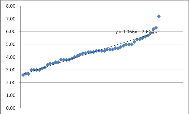
From the data, we can say that the 95% confidence interval that regression line is as follows:

The above shows a regression line of y = 2.614 + 0.066x while the graph below shows y = 2.709 + 0.066x.
Diagnostic
Heteroscedasticity
Heteroscedasticity is the relationship of the data which varies in a constant manner upon the introduction or change of a variable it is expressed in the following formula yt = βo + β1xt + β2zt +Et. In such regression Et represent a problem that shows the variable changes form tie to time in the equation xt and xz represents the variable that change in a constant manner. It is used to estimate the biasness in the data and the significance of the statistics (Engle 1982).
In other words heteoskedasticity is the variance of random error of a regression equation where there are variable that deviate from sample means. In other words heteroskedasticity is the variance of random error of a regression equation where there are variable that deviate from sample means (Kuttner 2001).
Heteroskedaticity occurs when variances of the data are not constant. It is always a problem of data from various cross-sectionals sources. It does not have any effects on parameters such as coefficients and means. Therefore it can be simply being described as the biasness of estimated parameters. The consequences of heteroskedasticity are that the data estimate becomes biased and constant the estimates are also not efficient relative to other estimates (Diamond and Jefferies 2000).
There are a number of test that are carried out heteroskedasticity, one of them is white and it takes the following form:
- the observation are made in ascending order.
- There is an assumption of positive relationship to one variable.
- Observation which falls between those which are large and low is omitted.
- Separate regression is carried out for the two observations to obtain respective residue some of squares.
Autocorrelation
Autocorrelation has a number of consequences that are to be considered. The first consequences of autocorrelation is that its coefficient are not biased meaning that the results obtained form the calculation about the standard errors of tow data sets are biased. In some instances it may have a large non serial figure which will lead to large error variances which makes the report that is subjected to autocorrelation be biased.

Normality
In order of one to collect heteroskedasticity numbers of procedure carried out this include:
- verification of variance and standard errors
- Making necessary assumptions relating to variance, standard errors, and an assumption that it is to transfer the original model through multiplying the data, by diving by the data. This is done through estimating regression line and then using the estimates to re-estimate the collective mode (Bryman 1992).
- A log transformation is used to transform the data.
- Some variable are dropped.
Unit root
Unit root test is a tool that is used in forecasting model such as ARIM models. It also shows the differences between stationary and non stationary of model, it considers the differences in data. The differences between stationery and non stationary are tested using this tool to guide decision making of a specific data. Mostly is used in economic, mathematics in trying to distinguish between samples of data. Unit root test always considers differences or non existence of differences which are used in the sample. All this depends on the processes, interest, sample sizes and properties of the tests (Bollerslev 1986).
From statistics little is known about unit root test as a forecasting tool in halve casting model. Most writers have used this tool in conjunction with Monte Caro studies which were used to explore the symmetry of the data. Unit root test is used and improves forecasts in various sample sizes various forecast horizons and degree persistence with the data (Rigobon and Sack 2004).
Dickey Fuller method of unity root testing is in two forms. The method involves simulating distribution in an elegant way (Bollerslev, Engle and Nelson 1994). It involves the five ways:
- Simulating distribution by random walk where Yt =yt-1 + Et where t =1..t
- Determination of the maximum value of the expected under the model of simulation.
- Determination of the maximum value of the expected function under hypothesis one
- Use the two values calculated in two and one to determine the LR test.
- The result is repeated now and again for purposes of simulation. This is the method that is used in unity root testing under Dickey Fuller method of unity testing.
Where total number of values is subjected to a division of the sum of each of the values being considered. It is an appropriate measure central tendency of a number of returns calculated for a particular time. However, when there is percentage changes in value over time are involved this figure can be misleading. Therefore the availability of continues compounded returns. This can be defined as the nth root of the product result from multiplying:
G = [(1 + R1) (1 +R2)…. (1 +Rn)]n -1
Where:
- R = total return
- n = number of periods.
Note that adding 1.0 to each return produces what we call a return relative. If the return for a period is 10 percent (.10), then the return relative is 1.10. The investor has received $1.10 relative to each $1 invested. If the return for a period is (-15) then the return relative is.85(-.15). Return relatives are used in calculating geometric average because negative total returns cannot be used in the math.
In determining whether two variables are integrated various tested are carried out to determine the cointegration. To beginning with, cointegration is a concept where two time series variables are determined and assumed to have been generated by non stationary. Cointergration is important in assisting non stationary economic series to become clear and understandable to users. The idea of cointegration is important and it uses statistical theories in estimating and testing. The data used in testing and estimating should have linear systems, which are coefficients of the statistical relationship within these values are known for unity root testing (Wongswan 2009).
Cointegration method is used to show how data in modeling is cointegrated. It is a useful tool for testing and estimating parameters with linear systems. It is used to integrate errors of non stationary variable in a regression error. The method of cointegration is used in empirical analysis especially in economics such as wealth consumption and it has made economic relationships easier. Cointegration integrates various models to arrive at unknown model. This method involves testing hypothesis and making autogressive model where they are considered in decision making (Bernanke and Kuttner 2005).
Changes in the bank rate influence other rates of interest. When bank rate is raised, borrowing becomes more expensive and demand for loans is reduced, thereby reducing purchasing power. Conversely a reduction in the bank rate will lead to an expansion of bank deposits. The resulting fall in overdraft rates will encourage borrowing, while saving will be discouraged because of the lower rate of interest paid on savings. Changes in the bank rate influences other rates of interest, when the discount rate is raised, borrowing becomes more expensive effectively reducing demand for loans, the resulting effect in the economy is reducing the purchasing power of people.

When the interest rate is increased there will be an increase in the cost of live. This will reduce the quantity demanded and consumed in the market.
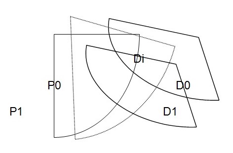
In the graph, D0 is the original demand curve if there is an introduction or increase of interest rate in the market, demand will reduce to D1. When demand reduces to D1 price will not remain the same, it will also change to P1 to create an equilibrium price at which the new demand D1 intersects the supply curve SS1. As a result of the increase in the interest rate, equilibrium amount demand and supply will also fall to OP1.
A rise in prices is harmful to the consumers’ interests. They have to pay more for everything that they buy. Their incomes do not go as they could go before.
Reference List
Bernanke, B., Kuttner, K., 2005. What explains the stock market’s reaction to Federal Reserve policy? Journal of Finance, LX (3), 1221-1257.
Bollerslev T., Engle R. F. and D. B. Nelson (1994), ARCH Models, Handbook of Econometrics Vol. 4
Bollerslev, T.P. (1986), Generalized Autoregressive Conditional Heteroscedasticity, Journal of Econometrics.
Bryman, A. (1992). Quantity and quality in social research 2nd Ed.
Diamond, I. & Jefferies, J. (2000). Beginning Statistics. An Introduction for Social Scientists. California: Sage Publications, 2000.
Engle, R.F. (1982), Autoregressive Conditional Heteroskedasticity with Estimates of the Variance of U.K, Econometrical.
Engle, R. F. (2001), GARCH 101: The Use of ARCH/GARCH Models in Applied Econometrics, Journal of Economic Perspectives.
Gracas, M., Colares, L. and Sandre-Pereira, G.(2001). “A Research on Nutritional Status of Brazilian Lactating Mothers”. Nutrition and Food Science, Vo. 31, No. 4, pp. 194-200.
Kuttner, K.,(2001). Monetary policy surprises and interest rates: evidence from the Fed Funds futures markets. Journal of Monetary Economics, 47, 523–44.
Rigobon, R., Sack, B.P., 2004. The impact of monetary policy on asset prices. Journal of Monetary Economics, 51, 1553-1575.
Wongswan, J., (2009). The response of global equity indexes to U.S. monetary policy announcements, Journal of International Money and Finance, 28, 344–365.
