Introduction
In microeconomics, the indifference curve is assumed to be the graph that shows diverse bundles of goods where each bundle is measured as to the quantity in which the consumer is indifferent. The major function of indifference curves is to represent demand patterns for individual consumers over bundles of commodities (Bruce & Jeffrey).
The indifference curve may be defined as a curve that joins all the possible combinations of two commodities that give equal satisfaction to consumers. A consumer can, therefore, easily know (according to his scale of preferences) what combinations of two commodities give him the same level of satisfaction.
The usefulness of the indifference curves:
- it helps to distinguish between the substitution effects and the incomes effects
- it provides an ordinal measurement of utility
- it helps to compare the satisfaction of different goods/commodities and enables the consumer to attain the equilibrium
- an indifference curve helps the consumer to determine whether he/she is attaining the maximum satisfaction or not.
Indifference curves aim at analyzing how a rational consumer chooses between two goods through combining both the indifference and budget line constraints. The axes represent goods and indifference curves are downward sloping (by assumption).
The good with a negative income elasticity of demand is regarded as an inferior good (i.e. its increased income leads to a fall in consumption for this good). On the other hand, a giffen good is seen as an inferior good of the extreme (resulting from a strong income effect) such that an increase in prices for this good results in increased consumption of the same. This means that the sales of inferior goods are counter-cyclical making companies that produce them also counter-cyclical/resistant to economic cycles
The normal good refers to a good in which consumers increase their demand on it whenever their incomes increase hence contrast with the inferior good in consumer theory since it decreases in demand when the income of consumers increases. The amount of a good bought can increase, decrease or remain constant since it depends on the consumer /market indifference curves.
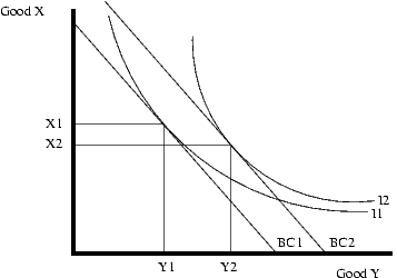
In the illustration below, the bus journey is viewed by commuters as an inferior good while the car journey is viewed as a normal good. The bus journey is plotted on the horizontal axis represented by good y while the vertical axis represented by good x is the bus journey. As shown in the diagram, good y is a normal good since the quantity purchased increases from y1 to y2 as the budget constraint shifts from BC1 to the higher income of BC2 i.e. income increases. On the other hand, good x is an inferior good since the amount demanded decreases from x1 to x2 as income rises with the same margin (John Gianakopulos).
A normal good will always respond positively to the changes in income whereby an increase in income will, in turn, result in a comparable increase (change) in demand for this normal good.
Ability to Buy-bus journey (deriving the curve)
This concept of deriving on indifference curve can be explained by the help of an example hence assume that the following combinations of bus and car journey travel fares were recorded:
Indifference schedule
Combinations bus car
1st 20 1
2nd 15 2
3rd 11 3
4th 8 4
5th 6 5
The above combinations can now be represented on an indifference curve. The car fare is recorded on the x-axis while the bus fare is recorded on the y axis. The points are marked on the curve that represents these combinations. The curve which joins these combinations is known as the indifference curve. The higher curves will give more satisfaction while the lower curves give less satisfaction.
Income is a very critical factor that certainly determines the ability to purchase a given commodity.i.e. higher purchasing power is tied with higher income and the opposite is true.
A change in the income implies a shift (rightwards or leftwards) in the demand curve as indicated in the above diagram.
An increase in income will translate into increased demand (i.e. a rightward shift of the demand curve for transport) whereas a decrease in buyers’ income will translate into a reduction in demand (demand curve’s leftward shift). The income elasticity of demand (which is a relative response of demand to income changes) of a normal good is positive (greater than zero) while inferior good has a negative income elasticity (less than zero) (Volker & Hans).
Price changes
Substitution effects
This is the overall effect arising from changes in the relative prices of commodities. The diagram below shows the resultant effect after an increase in price for good y. An increase in price for good y leads to the budget constraint pivoting from BC2 to BC1. The price of x is not changing and the buyer can as well purchase the same quantity of x. Consequently, if the consumer opts to buy good y then he will be forced to buy less as a result of an increase in price in this good.
For utility maximization with the reduced budget constraint (BC1), the customer will be forced to reallocate consumption to achieve the highest available indifference curve to which BCI is tangent to. As the diagram demonstrates, the curve is l1, and thereby the amount of good y purchased will as a result shift from y2 to y1, and the amount of good x purchased will shift to x1 from x2. Consequently, the opposite effect will be true if the price of y decreases i.e. it will cause the shift from BC2 to BC3 and l3 to l2.

Income effects
The income effect of consumers also changes with income changes. It’s a phenomenon observed through changes in the purchasing power and it reveals the change in quantity demanded brought about by a change in real income level/utility. With constant prices, any change in income will graphically imply a parallel shift in the budget constraints. Increasing the income will shift the budget constraint right since more of both can be purchased and reducing income will shift it leftwards as indicated in the following diagram.

Explanation of the substitution and income effects of a price change
When the price of one commodity falls, the equilibrium of the consumer changes as a result. Due to the fall in the price of any commodity, the consumer can purchase the same quantity of each commodity as he/she did before the fall of the price of that commodity and have some money left over. It is called the income effect because the increase in the purchasing power of the consumer due to the fall in the price of one commodity is due to the reason that his/her income has increased.
When the purchasing power of the consumer rises due to the fall in the prices of one commodity, the consumer must decide how this increase in the purchasing power is to be spread over the different goods that he purchased. The consumer will always reallocate his expenditure in such a way as to purchase relatively more of commodity x whose price has fallen and less of commodity y. The second force is called the substitution effect; Substitution means the change in the quantity of a commodity purchased only due to the change in the relative prices. The income and the substitution effects are explained in the diagrams above.
BC1 is the price line when money at the disposal of the consumer is assumed to be $10 and the price of x and y commodities are $2 and $1 per unit respectively. The consumer is in an equilibrium position at point p. now we assume that the price of x commodity falls from $2 per unit and to $1 per unit. The consumer’s equilibrium point changes from p to p1. The movement of the consumer from point p to p1 as a result of a fall in x commodity is in reality a result of the two forces. When the price of x commodity falls, the consumer will feel that now he/she is in a better position as he/she can purchase the same quantity of both commodities and have some money left over. It is as if the prices of the same commodities remained the same and the consumer’s income had gone up. At the new equilibrium of p1, the consumer will experience more satisfaction as compared to point p i.e. original equilibrium. The consumer could achieve the same satisfaction if his/her income had increased in such a way that the new price line could be tangential to IC2 at the point of intersection (Volker & Hans).
In the diagrams above, at point p (initial equilibrium) consumer purchases three units of x commodity and at point t (intersection point) he/she purchases four units of x commodity and at point pi (new equilibrium) he purchases six units of x commodity. When due to a fall in the price of x commodity more units of x commodity are purchased, the increased purchase of x commodity is the result of the income effect and the substitution effects. The substitution effect is equal to the change in the purchase of x commodity minus income effect. It can be expressed as:
Price effect (PE) = income effect (IE) + substitution effect (SE)
In the diagram, the curve that joins original equilibrium (p) and the point of intersection (t) is known as the income consumption curve and the curve which join point p and p1 is called the price consumption curve. These curves help to determine the substitution and the income effects.
Altered tastes
When the bus journey tastes changes and is no longer viewed as an inferior good (may be due to the improved services that they are offering), the consumers would be able to increase demand for it when their incomes increases and cut on their demand for it when the incomes reduce. It basically becomes a normal good and the illustrations made earlier would be applicable in this case. The diagram below indicates good y (bus transport) to be a normal good since its demand increases with an increase in income.

Work Cited
- Bruce R. Beattie and Jeffrey T. LaFrance, “The Law of Demand versus Diminishing Marginal Utility”. Review of Agricultural Economics. (2006), pp. 263-271.
- John Geanakoplos. “Arrow-Debreu model of general equilibrium, “The New Palgrave: A Dictionary of Economics, (1987) v. 1, pp. 116-24.
- Volker Böhm and Hans Haller. “Demand theory,” The New Pal grave: A Dictionary of Economics, (1987) v. 1, pp. 785-92.