Supplemental Fiscal Budget and Capita Gross Domestic Product

Introduction

The government of developing nation X is prepared to allocate $2 billion in support of policy measures to grow per capita Gross Domestic Product (GDP) in the medium term, over a fifteen-year period. The two policy measures under scrutiny:

1. devote the earmarked funding to raising the secondary school enrolment rate (the percentage of the secondary school age population) from 55% to 61% in the same time span; or
2. emergency loans for the banking sector to forestall a drastic drop in the ratio of Private Credit by Deposit Money Banks and Other Financial Institutions to GDP to 0.38 versus 0.52 currently.

For the rest of this paper, the task is to employ an empirical model to test which of the two policy measures will enable country X, ceteris paribus, to attain greater appreciation in per-capita GDP.

Data Transformations

Item 1

The compiled data is shown in Table 1.

Table 1: Compilation of Logged and Calculated Data

The Empirical Model and Tests of Hypotheses

The result of the specified model based on the calculated coefficients in Table 2 (below) is as follows:

dlypc_i = β₁ + β₂lypc90_i + β₃lseced_i + β₄govgdp_i + β₅open_i + β₆infl_i + β₇credit_i + u_i

dlypc_i = 1.59 – 0.92 (lypc90) + 0.58 (lseced) + 0.26 (govgdp)+ 0.10 (open)+ 0.38 (infl)+ 0.39 (credit)

Table 2: Calculated Coefficients

a. Dependent Variable: PCI ch 1990 to 2005

Item 2i

Table 3 (below) presents the ANOVA results for the model as a whole and therefore constitutes a test of the hypotheses H0:b2=b3=b4=b5=b6=b7=0 against H1:bj=0. The F value is so high as to yield a significance statistic p < 0.05. This means the non-zero beta coefficients could have occurred by chance alone perhaps three times in a hundred country data compilations. One must therefore reject the null hypothesis.

Table 3

a. Predictors: (Constant), Ratio private credit to GDP 1990, Openness of the economy, Govt share real PC GDP 1990, Inflation rate 1985 to 1990, Ln Secondary enrolment 1990, Ln PCI 1990

b. Dependent Variable: PCI ch 1990 to 2005

Item 2ii

When each of the independent variables is tested singly, the result for the variable lypc90 (the log transformation of per-capita GDP in 1990 for all countries involved in the analysis) is that β₂ rises from -0.915 in the multiple-regression model to -0.036. However, the t test associated with this beta coefficient is so low (-0.25) that the significance statistic p = 0.81 fails the minimum hurdle of a 95% confidence level. The outcome for the single-IV hypothesis test (Table 4 overleaf) is at the same unsatisfactory level. The F value for β₂ is so low that this result could have been obtained roughly once in every five times a random selection of nations is compiled. This means that we cannot reject the null hypothesis. The log transformation of per-capita GDP in 1990 does not, by itself, predict the rise from 1990 to 2005 embodied by the logged value dlypc.

Table 4: Hypothesis Test Result for β₂

Item 2iii

Performing the same single-IV test with the variable seced (the proportion of the secondary school age population enrolled in 1990), one finds that the value for β₃ drops from 0.577 in the multiple-regression model to 0.052. The t test associated with this beta coefficient is so low (0.35) that the significance statistic p = 0.73 also fails the minimum hurdle of a 95% confidence level. The outcome for the single-IV hypothesis test (Table 5 below) is also just as dismal. The F value for β₃ is so low that this result could have been obtained roughly once in four times a random selection of nations is compiled. This means that once again, we cannot reject the null hypothesis. The log transformation of secondary enrolment rate as of 1990 does not, by itself, predict the rise from 1990 to 2005 embodied by the logged value dlypc.

Table 5: Hypothesis Test for Logged SECED

a. Predictors: (Constant), Ln Secondary enrolment 1990

b. Dependent Variable: PCI ch 1990 to 2005

Item 2iv

Performing the same single-IV test with the variable credit (ratio of private credit by deposit money banks and other financial institutions to GDP in 1990) and on a less stringent 90% confidence level, one finds that the value for β₇ drops from 0.390 in the multiple-regression model to just 0.109. The t test associated with this beta coefficient is so low (0.76) that the significance statistic p = 0.45 is virtually the same as even odds, the classic case of the random-outcome coin toss. The outcome for the single-IV hypothesis test (Table 6 below) is also just as dismal. The F value for β₇ is so low that this result could have been obtained virtually every other time a random selection of nations is compiled. Once again, we cannot reject the null hypothesis. The ratio of private-sector credit to local GDP as of 1990 does not, by itself, reliably predict the rise from 1990 to 2005 embodied by the logged value dlypc.

Table 6: Hypothesis Test for Ratio of Private-Sector Credit to GDP as of 1990

a. Predictors: (Constant), Ratio private credit to GDP 1990

b. Dependent Variable: PCI ch 1990 to 2005

Item 3: Implications for Allocation of $2 Billion According to the Base Empirical Model

All other macroeconomic and political factors held constant, allocating the new money to supporting private loan activity has more immediate, far-reaching and significant impact on per-capita incomes.

Since the “stimulus funding” of $2 billion can go one way or the other, we first of all set aside the credit variable, re-specify the empirical model as shown below, recompute and input average values for the five known macroeconomic variables…

dlypc_i = β₁ + β₂lypc90_i + β₃lseced_i + β₄govgdp_i + β₅open_i + β₆infl_i + β₇credit_i + u_i

dlypc_i = 1.01 – 0.515 (lypc90) + 0.408 (lseced) + 0.222 (govgdp)+ 0.044 (open)+ 0.394 (infl)

dlypc_i = 1.01 – 0.515 (8.49) + 0.408 (0.61) + 0.222 (16.14)+ 0.044 (47.93)+ 0.394 (0.1)

Note that the value for SECED has been inputted as the goal of 61% of the applicable secondary-age population.

Assuming that the new funding goes to classrooms and salaries for new teachers and that the capacity to accommodate a 6 percentage point increase in secondary school enrolment is in place right when the regular school term opens in year 1, the result would be a mean rise of 2.62% in per-capita GDP every five years. Over a 15-year time span, a developing nation that made the special, one-time investment in public education might therefore expect a cumulative 10.5 percent gain in population-adjusted income. However, this model explains just 8% of the variance in the expansion of per-capita income over a 15-year span.

Allocating the money to prevent the collapse of private-sector credit means re-specifying the model by replacing seced with credit. The recalculated model is as follows:

dlypc_i = 0.925 – 0.40 (lypc90) + 0.235 (govgdp)+ 0.12 (open)+ 0.39 (infl) +.33 (credit_i)

dlypc_i = 0.925 – 0.40 (0.849) + 0.235 (16.14)+ 0.12 (47.93)+ 0.39 (0.1) +.33 (0.405)

In point of explaining a marginally higher proportion of total variance (9.4 %), the diversion of funds to sustaining private credit activity looks better. All other things equal, it is likely that a fresh infusion of $2 billion in private-sector credit will raise the available stock of loans and investments, spur jobs creation and generate demand for both capital and consumption goods. Hence, it is possible to foresee annual gains in per-capita GDP in the order of 2% and, for the 15-year period targeted, around 30.9%.

The Diagnostic Tests

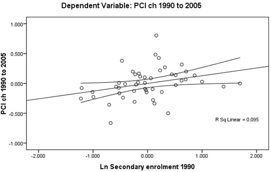
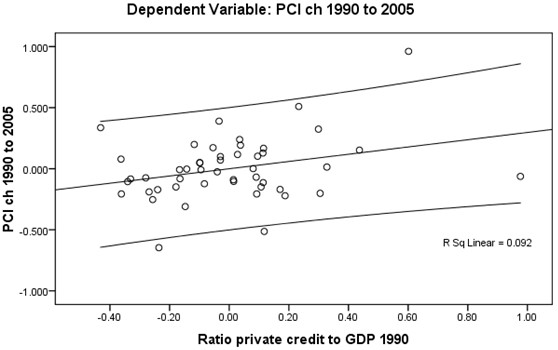
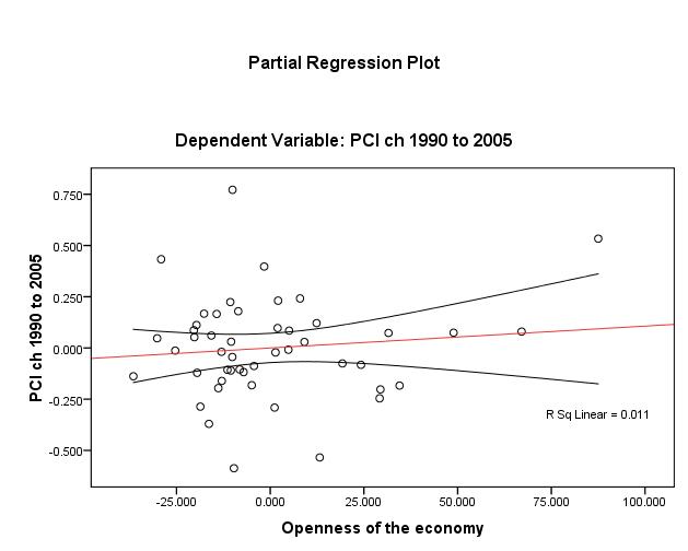
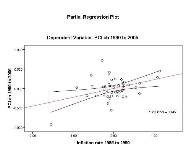
The test of the linearity assumption between Y (dlypc_i ) the two main IVs is best visualized by plotting (Figures 1 and 2 overleaf). A positive linear relationship exists though it is rather weak in both cases (unadjusted R₂ ≈ 9%) and the spread around the mean of credit is wide.

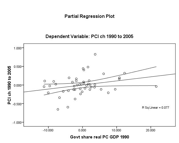
Proceeding to the three other independent variables (Figures 3 to 5 below), one discerns that the linear relationship is weakest for openness (unadjusted R₂ ≈ 1%). Nonetheless, one may assert that the linearity assumption is satisfied for all β_i.

On a basic level, the homoscedasticity assumption is satisfied by the fact that all the variables are continuous, either interval or ratio. This holds even when dummy variables are employed (see section 5 below) so long as these are done for the independent variables.

Besides simple visualization with boxplots, the classic method for testing homoscedasticity rests Levene’s statistic for the test of homogeneity of variances. For convenience, the dependent and key independent variables are categorized into quartiles (see Table 7 below). Table 8 then shows that:

• For the dependent variable, variance is narrow in the middle of the distribution but is wider at both upper and lower extremes of the distribution.

Table 7: The Quartiles

Table 8

• For the logged secondary school enrolment rate, variance is lowest in the second quartile and greatest for those nations with the least propensity for schooling in the secondary-school-age population.
• And for credit, variance is low in the lower half of the distribution but five times higher in the fourth quartile.

Hence, the original model does not meet the test for homoscedasticity of variances. Since this distorts the significance tests and affects external validity, it becomes very difficult to generalize from the original model.

Turning to the assumption of normality of distribution for the residuals, one finds that subjecting the relationship between DV and the seced IV with the one-sample Kolmogorov-Smirnov Test (see Table 9 below) for small to medium samples (in this case, n = 50) that: a) There are numerous cases of the Lilliefors Significance Correction when the change in per-capita GDP from 1990 to 2005 is constant at certain values od the DV; and, b) testing the limit of the theoretical cumulative normal distribution against the obtained distribution of residuals yields significance statistics p < 0.001 or lower. Hence, the assumption of normality for the residual distributions cannot be met.

Table 9

Relating dlypc to credit generates 100% Lilliefors Significance Correction exception warnings. The assumption of normality cannot even be evaluated.

Re-estimation with Dummy Variables

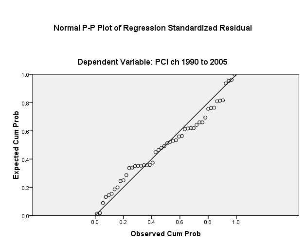
Given the calculated residuals for the regression, the 3X SE hurdle comes to 8.991. The probability plot (Figure 6 overleaf) shows, however, that there is no need to undertake the outlier-adjusted model specification.

Table 10