Executive Summary
The purpose of this management report will be to critically examine the main theories of international financial management and assess the extent to which these theories can be used in the real world. This will be a critical examination of any empirical evidence that exists on the theories used to explain international financial management which include the fisher effects theory, international fisher effects theory, purchasing power parity theory, Mundell-Fleming model theory, optimum currency area theory and the interest rate parity theory. The report will evaluate these theories based on their applicability to real world situations and offer suitable recommendations that will be used to improve the performance of these theories to international finance activities.
Introduction
The field of economics also assesses capital flows of financial information as well as international investments and trade deficits (Siddaiah 2010). The theories that are used to explain global finance in terms of swap rates, interest rates, money supply and demand which will be analyzed in this information include the purchasing power parity (PPP), the optimum currency area (OCA) and the Mundell-Fleming replica theory (Madura 2008).
Mundell-Fleming Theory
The main argument behind the Mundell-Fleming model is based on the fact that an open economy is unable to maintain a fixed exchange rate system which will have an effect on independent monetary policies (Mundell 1963). The traditional model of Mundell-Fleming is made up of the following equations: Y= C+I+G+NX (the IS curve)
- where Y is GDP, C is consumption, I represents investment, G is government spending and NX represents net exports
Another equation used by the Mundell-Fleming model is M/P= L (I, Y) (the LM curve)
- where M represents money supply, P is average price, L is liquidity, i is the interest rate and Y is the GDP
The components that make up the IS curve include consumption (C), gross domestic product (GDP), taxes (T), interest rate (i), investment (I), government (G) and net exports (NX). One important assumption of the model is that there is equalization of the local and global interest rates (Mundell 1963). Under a flexible exchange rate regime where the exchange rate is determined by market forces, any increase in money supply affects the local interest rates which in turn lower the local currency’s exchange rates. Exchange rates in foreign countries will be high leading to the flow of money out of the country thereby depreciating the value of the local currency. This depreciation in turn leads to a decrease in price of local goods which are sold at a relatively cheaper price when compared to foreign goods (Blanchard 2006).
The effect the depreciated currency has on net exports is that imports into a country will decrease while the exports will increase because of the decrease in prices for locally produced goods. The balance of payments is also meant to shift to reflect the depreciation of the local currency as the increase in the net exports (Mundell 1963). While considering the equality of the local and global interest rates, any increases in government spending will increase local interest rates resulting in an increase of money coming into the country. A stronger local exchange rate will increase the price of local goods and decrease the cost of foreign goods. This will lead to an increase in imports and a decrease in net exports lowering the number of goods exported to other foreign countries (Mankiw 2007).
A situation where the government controls the exchange rates is referred to as the fixed exchange rate regime where fluctuations in money supply are dealt with by the main monetary authority within a country. Any changes in regime spending will add to interest rates thereby leading to an increase in the swap rates (DeGrauwe 2000). Because the government controls the exchange rates, foreign currencies are purchased by the governing authority to reduce the pressure that is caused by increasing interest rates (Gamber and Colander 2006). The graph below depicts changes in money supply and government spending under the fixed exchange rate regime.

The Mundell-Fleming model has had a tremendous impact on the amount of research that has been conducted on exchange rate theories and also international financial management. Empirical evidence conducted on the model revealed that the Mundell-Fleming model assumed static expectations despite the existence of regressive or rational expectations and perfect foresight. Under the assumption of perfect foresight, there will be fluctuations in exchange rates which will have an effect on the domestic consumer price level which allows for more price generality. The empirical testing of the model under the perfect foresight assumption revealed the equation for the Mundell-Fleming model to be; ṡ =i – i* where ṡ is the domestic price of foreign currencies, i and i* represents both the domestic and foreign interest rates (Sarno and Taylor 2002).
Because the Mundell-Fleming model is log-linear, under the perfect foresight assumption, the model basically embodies the Keynesian theoretical framework where output is determined primarily by demand where any discrepancies between aggregate demand and supply lead to an adjustment in demand. Aggregate demand under perfect foresight is seen to be a function of an autonomous component (net export demand) and an interest-rate-sensitive component (investment or consumption) that is mostly influenced by international competitiveness. Empirical testing of the theory in the Keynesian analysis has revealed that aggregate demand under perfect foresight can also be a function of output (Sarno and Taylor 2002).
The exchange rate movements in the perfect foresight assumption will have a bigger effect on aggregate demand when compared to the effect posed by interest rates. There is empirical evidence that suggests private consumption and investment expenditure are insensitive to the interest rate movements as explained by Taylor (1999 cited by Sarno and Taylor 2002) meaning that the aggregate demand will be very small. If such a condition is satisfied, exchange rate system will have a unique convergent saddle path because the aggregate demand will be small.
Under such an assumption, the economy of a country will always be on a saddle path given that agents of a free economy are unwilling to participate in such an economy. The exchange rate will therefore go up to reflect the response to price shocks caused by the saddle path. In the IS-LM curve, the exchange rate will jump above its long-run equilibrium so that it can be able to get on its new saddle path, adjusting the output so that the economy is able to move along the saddle path to the new long-run equilibrium (Sarno and Taylor 2002). The diagram below represents the saddle path solution to the perfect foresight Mundell-Fleming model.
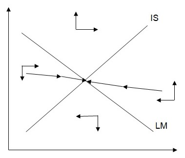
The use of the Mundell-Fleming model in real world applications has been criticized because of the inconsistency and irreconcilability of the various concepts that make up the theory. This presents a lot of inconsistency when trying to determine the local and global interest rates that will be charged on capital outflows on the exchange rate. Exchange rate flexibility is critical especially in the financial market of a country as they provide long-run multipliers to the economy. The inconsistencies in this model therefore make it difficult to develop long run multipliers that will be used to regulate money supply (Blanchard 2006).
To explain this further, in a financial market that utilizes the fixed exchange rate system with perfect capital mobility, the monetary policies that are in place become ineffective causing an outward shift of the LM curve leading to an out flow of capital from the economy. In such a case, the monetary authority charged with maintaining the fixed exchange rate system would have to sell its foreign currency so as to increase the reserves for domestic currency. The selling of foreign money to increase domestic currencies reduces the real balances that exist in the economy meaning that the use of this model in real world situations leads to inconsistent results (Mankiw 2007).
Optimum Currency Area (OCA) Theory
The optimum currency area theory basically refers to a large geographical area that utilizes a single currency so as to capitalise on economic efficiency. OCA describes the optimal characteristics that are needed to merge particular currencies or create new currencies whether or not a particular region is ready to become a monetary union. An optimal area of currency is usually larger than the total geographic area of a country as it is meant to cover every location that is under the common currency. The European Union is a good example of an optimum currency area that is covered by a single foreign exchange currency, the Euro (Baldwin 2004).
Robert Mundell developed the OCA theory based on two models economic models which included OCA with stationary expectations and OCA with international risk sharing. The first model OCA with stationary expectations is the most used by financial economists and countries under a common currency such as Europe where asymmetric shocks are used to undermine the functions of the real economy. If these asymmetric shocks are deemed to be uncontrollable and too important to ignore, then the monetary authority has to consider a regime of floating interest rates which will be difficult to adjust to suit the needs of individual regions (Frankel and Andrew 2001).
The criteria that is used to identify successful currency unions under the OCA theory include labour mobility across the regions where individuals can be able to move across a country’s border and not have to convert their local currency to that of the other country. The absence of barriers that prohibit free movement across borders is also another important criteria that is used to identify currency unions as well as the existence of institutional arrangements that to cater to superannuation transferability across borders. Openness with capital mobility and flexibility of wages across regions is another important criterion for optimal currency areas because it influences the automatic distribution of money and goods to areas where they are needed. The third criteria for OCA is a risk sharing system between countries such as an automatic fiscal transfer means that reorganizes cash to areas that fall under OCA (Ricci 2008).
The final criterion requires that participant countries should have similar business cycles where in the event one country in the optimal currency area experiences a recession or economic growth the rest are meant to experience the same effect. The OCA with statutory expectations model has mostly been applied in the European Union and in the United States (Kouparitsas 2001). The second model OCA with international risk sharing deal with the uncertainty that is brought about when exchange rates interfere with the economy of a country. This replica varies with the preceding one in that asymmetric jolts inside the financial system are not believed to destabilizing the ordinary legal tender in that the claim that all regions have on the currency (Mundell 1961). The diagrams below represent the GG and LL schedules that explain the changes in optimal currency areas.
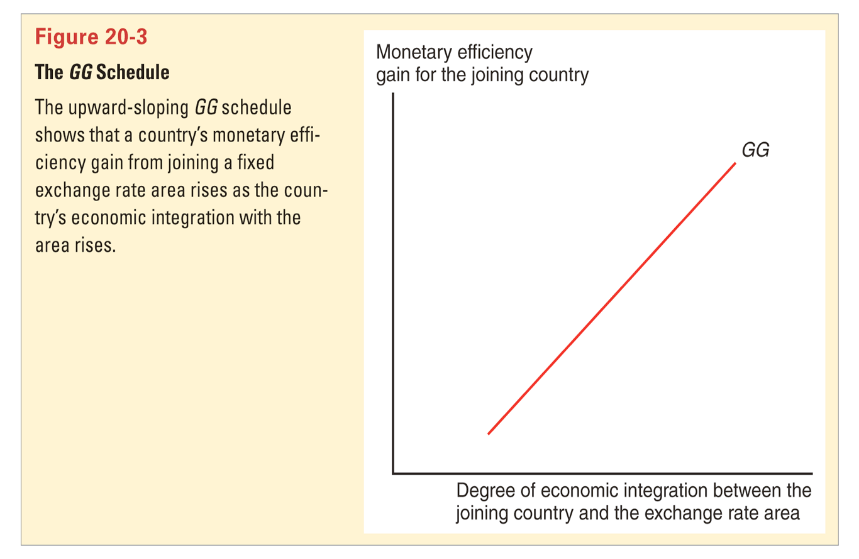
The graph represents the monetary efficiency gai economic integration. The members of the common currency are assumed to have a stable price level.
The real life application of the optimal currency area as mentioned earlier on in the discussion is mostly in the European Union where many of the member states have adopted the Euro as the common currency. While many have seen the common currency to be beneficial to the European Union because it has led to a stable and strong local currency, many economists have criticized the Euro in terms of its flexibility to other exchange rate currencies in the world (Wray 2000). With regards to the empirical testing of this theory, there have been few systematic tests that have been developed to support the OCA theory as a useful technique of explaining similar currency areas. The rarity of changes in currency areas during the 1970s and 80s made it difficult to conduct any empirical tests on this theory. It is only recently with the currency changes in Europe that theorists sought to test this theory to determine whether it could be applicable to a large geographic area (Janicki et al 2005).
Janicki et al (2005) conducted an empirical testing of the optimal currency area theory by using a gravity model to test the applicability of the theory to real world situations. The researchers tested the theory by using bilateral FDI flows instead of bilateral trade where FDI flow is the movement of production activities across borders. They did this so that they could be able to measure Mundell’s argument about the allocation of capital flows to support the use of a common currency within one geographic location. The bilateral FDI flows were therefore use to empirically test the theory instead of capital flows while exchange rates were considered as other variables.
Janicki et al (2005) made use of the gravity model which is commonly used in international trade and financial management to analyse the FDI bilateral flows. The model estimates international trade by considering market size, factor endowments and income similarities within certain geographic locations. The gravity model in this case incorporated all of these aspects as well as proxies that would be able to capture the European convergence to create the Euro currency. These proxies included the inherent differences that existed in interest rates, debt differences as well as budget differences within the European Union. The variables that would be used to explain the model took the following forms:
- Gij,t = 1n(Yit + Yjt ) and
- Sij,t = 1n[1- (Yit / Yit + Yj ) – (Yjt / Yit + Yj )2 ]
G represents the overall economic space that will be measured by the proxy of market size which also represents investment and S represents an index that is meant to capture the relative size of two economies. The flow of FDI in these equations is characterised by cross-border investments where investors in different geographic locations have a long-term interest in other economies under the optimal currency area. Janicki et al’s (2005) state that; “test revealed that bilateral FDI flows within the OCA theory could be explained by characteristics such as high-income consumer markets and also structural stability”.
The findings were therefore in line with the current theory for optimal currency area where low interest rates, capital and labour mobility, free movement across borders, reduced budget deficits and limits on government spending determined whether countries under one optimal area would fall under one currency. The convergence of two theories based on the empirical analysis of the theory with regards to a country’s income was seen to positively increase bilateral FDI flows where multinational companies preferred to invest in countries that had a similar economic and market size such as that in Europe (Janicki et al 2005).
Purchasing Power Parity
Purchasing power parity is deals with the relative price levels that exist in similar commodities that are sold in two countries. The theory seeks to explain how these relative price levels affect the long term equilibrium of exchange rates and the local currencies used in the two countries. The main assumption that underlies the purchasing power parity theory is that identical goods will have the same price in different countries or markets is they are sold under one common currency (Krugman and Obstfeld 2009). The purchasing power parity is based on three assumptions which include the law of one price, the free role of arbitrageurs and the unrestricted movement of goods or financial assets between two countries (Kevin 2009).
The law of one price states that the prices of identical goods and financial assets that can be traded are within the transaction cost of equality. The free role of arbitrageurs allows them to take advantage of the disparities in product prices anywhere in the world. The unrestricted movement of goods or financial assets explains purchasing power parity to be a lack of any restriction for the movement of goods and financial assets (Kevin 2009). These assumptions are used to explain PPP as the type of rate that is placed on two exchange rates based on their purchasing power. The purchasing power is basically the amount of goods and/or services that can be purchased with a unit of currency (Kevin 2009). For example if a watch costs Rs. 90 Indian Rupees and $2 US dollars, the equilibrium exchange rate between the dollar and the rupee will be $2 US= Rs.90. If the cost of the watch increases to Rs.99 based on a 10 percent increase in inflation, the exchange rate between the Indian Rupee and the US dollar will adjust to equate the purchasing power of the two currencies (Kevin 2009).
The purchasing power parity theory is made up of two models the first of which the absolute version which states that the exchange rate between the currencies of two countries is equal to the ratio of the price levels of the two countries based on the respective consumer price indices (Madura 2008). This is represented by the equation; eo = Ph / Pf
- where eo represents the current exchange rate, Ph represents the price level in the home country and Pf represents the price level in the foreign country
The absolute version determines the exchange rates between two currencies but it is only useful in the event similar commodities are included in the same proportion of goods being used for the calculation of the price level. The relative version of PPP is used to explain how exchange rates fluctuate by postulating one of the factors leading to exchange rate fluctuations to be inflation which affects respective countries meaning that the rate of inflation equals the differential rate of two countries. If the inflation rates between the two countries remain equal, the exchange rate between the currencies will not be affected and if there is a deviation, the exchange rate will be adjusted to reflect the inflation rate between the two currencies (Mankiw 2009). The relationship between the change in exchange rates and the inflation rates is expressed by following equation:
- e t = (1 + i h,t)t where et = expected exchange rate at time period t
- e o (1 + i f, t)t e0 = current exchange rate
- ih,t = expected domestic inflation rate at time period t
- if, t= expected foreign country inflation rate at time period t
A lot of empirical research has been conducted on the validity of the theory with most of these studies presenting conflicting information on the applicability of the theory to real world applications. Some of these studies have failed to examine the long-run relationship that exists between exchange rates and the price of domestic commodities within a certain economy. These studies have also concentrated on using data from advanced industrialized countries instead of developing countries which leads to conflicting information on the validity of the theory to real world situations. Islam and Ahmed (1999) conducted an empirical examination of the purchasing power parity theory by using causality and co-integration tests such as the Granger test that were based on the exchange rates of Korea and the United States. The researchers made use of time series data that was qualitative in nature based on data series collected from 1971 to 1996 (Islam and Ahmed 1999).
The researchers were able to examine the causal relationship that exists between exchange rates, domestic price levels and foreign prices of domestic products through the use of the Granger test. The test evaluated the causal relationships that existed between the mentioned variables where the bi-variate causal relationships included the causality between exchange rates and the relative price of domestic products in Korea compared to those in the United States. The results of the test revealed that there was a relationship between the Korean exchange rate and the foreign price level of commodities in the United States (Islam and Ahmed 1999).
The Granger test also revealed that there were causal relationships that existed between the exchange rates of a country and the relative price of products within the same country. The co-mixing tests that were used to gauge the strength of the purchasing power equality theory revealed that the short-run dynamics in the Korea-US currencies demonstrated that the exchange rate was a stable function of the relative price level of foreign exchange rate adjustments of 24 percent within one year. Islam and Ahmed’s study however showed a partial support of the purchasing power parity theory in explaining the domestic price levels of commodities in the country and the exchange rate of the American dollar (Islam and Ahmed 1999). The Granger and co-integration tests revealed that nominal exchange rates and price levels within the country were not stationary which depended on the differences in economic growth and market size in both countries. The researchers however supported the hypothetical framework of the PPP theory in explaining the long-run equilibrium between domestic prices and exchange rates (Islam and Ahmed 1999).
Recommendations and Conclusion
While the evaluated theories have a strong foundational basis, various aspects of these theories need to be re-evaluated to ensure they can be applicable to various economic situations. For example, the inconsistencies in the concepts that make up the Mundell-Fleming model need to be revised so that they can be applicable to determining the relationship between local and global interest rates. The various political issues that arise when the optimum currency area model is developed also need to be addressed to ensure that the model is able to incorporate the political structures of these countries. For the purchasing power parity, price structures for different goods need to be developed to explain the local and foreign exchange rate currencies of products sold in various countries.
Such revisions to these international finance theories will involve conducting more research and empirical testing to determine whether the theories can be adjusted to reflect real world economic problems such as exchange rates, different currencies and differing commodity prices around the world. The report has basically provided important empirical evidence on the various theories that can be used to measure international financial management concepts in use in various economic contexts.
References
Baldwin, R., (2004) The economics of European integration. New York: McGraw Hill
Blanchard, O., (2006) Macroeconomics, 4th Edition. New Jersey: Prentice Hall
DeGrauwe, P., (2000) Economics of monetary union. New York: Oxford University Press
Frankel, J.A., and Andrew, K., (2001) The endogenity of the optimum currency area criteria. The Economic Journal, Vol. 108, No. 449, pp 1009-1025
Gamber, E., and Colander, D.C., (2006) Macroeconomics. Cape Town, South Africa: Pearson South Africa
Inter Economics (2009) Optimum currency areas and the European experience. Currency Unions-1. Web.
Islam, A.M., and Ahmed, S.M., (1999) The purchasing power parity relationship: causality and co-integration tests using Korea-US exchange rate and prices. Journal of Economic Development, Vol.24, No.2, pp 95-111
Janicki, H.P., Warin, T., and Wunnava, P.V., (2005) Endogenous OCA theory: using the gravity model to test Mundell’s intuition. Center for European Studies, Working Paper No. 125. Web.
Kevin, M., (2009) Fundamentals of international financial management. New Delhi: PHI Learning Private Limited
Kouparitsas, M.A., Is the United States an optimum currency area? An empirical analysis of regional business cycles. Federal Reserve Bank of Chicago Working Paper 2001-21
Krugman, P., and Obstfeld, M., (2009) International economics. California: Pearson Education
Madura, J., (2008) International financial management. Mason, Ohio: Thomson Higher Learning
Mankiw, N.G., (2007) Macroeconomics, 6th Edition. New York: Worth Publishers
Mankiw, N.G., (2009) Principles of economics. Mason, Ohio: Cengage Learning
Mundell, R.A., (1961) A theory of optimum currency areas. American Economic Review, Vol.51, No.4, pp 657-665
Mundell, R. A., (1963) Capital mobility and stabilization policy under fixed and flexible exchange rates. Canadian Journal of Economic and Political Science, Vol. 29, No. 4, pp 475–485
Ricci, L.A., (2008) A model of an optimum currency area. Open-Assessment E-Journal, Vol.2, No.8, pp 1-31
Sarno, L., and Taylor, M.P., (2001) The economics of exchange rates. Cambridge, UK: Cambridge University Press.
Siddaiah, T., (2010) International financial management. New Delhi, India: Pearson Education India
Wray, L.R., (2000) The neo-chartalist approach to money. Working Paper No.10. Web.