Shuzworld: Assessment of Plant Operations

Date:
To: Production Manager
From:
RE: Assessment of Plant Operations

Purpose of Memo

The purpose of this assessment is to achieve the following:

1. Recommend the best method to be used by Shuzworld in sneaker’s manufacture. The options available are:
   1. Use of reconditioned equipment
   2. Purchasing new equipment in Shanghai Plant.
   3. Outsourcing to another manufacturing operation.
2. Develop a sales volume forecast. The results of the methods used are compared against each other. The methods used include:
   1. Least square method
   2. Trend Adjusted Exponential Smoothing
3. Discussion of application of control chart metrics in quality improvement at Shuzworld production line.

The best method for Shuzworld in sneaker’s manufacture

Manufacturing often calls for complex decision-making processes. When a number of options are at available, facts are necessary in order to come up with the best method to adopt (Brodd, 2005). In this analysis, break even method was chosen

Based on this method, at break even point, the value of sales equals the value of foxed costs added to variable costs. This is summarized by the equation below:

Calculating profits based on this method involves this equation

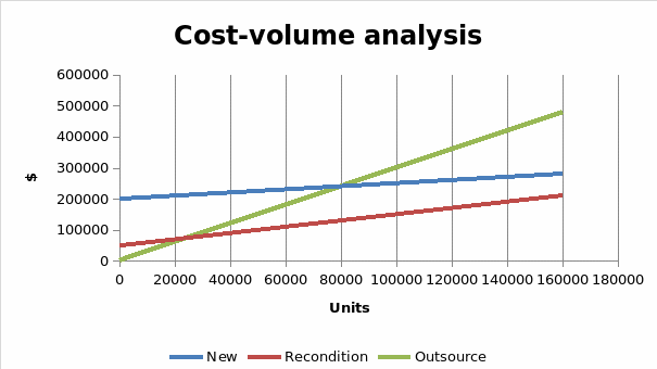
On basis of this equation, at break-even point, the profit values are equal to zero. This provides the basis for comparison of different production approaches to be employed by Shuzworld. The method was chosen for use in this analysis due to its ability to examine the relationship between costs, production, product volumes and the anticipated returns. Additionally, it allows managers to establish the effect of changes in fixed costs, variable costs, and price of commodities on revenues (Brodd, 2005). Based on these calculations, an Excel break-even analysis tool was used to generate the following results:

Comparing new plat acquisition against reconditioning o f the existing plat yields a break-even point at 300,000 units and 350,000 dollars. Comparing new plant acquisition against outsourcing yields a break-even point at 80,000 units and $240,000 while a comparison of reconditioning against outsourcing yields a break-even point at 25,000 units and $75,000. Based on the graph points obtained for cost-volume analysis, while outsourcing will cost less to manufacture 1000 units, higher production units like 160,000 would favor acquisition of a new plant. For high production rates, the best option would be to acquire a new plant. The scenario is best illustrated by the graph below:

Sales-Volume Forecast

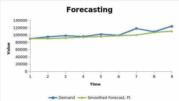
Accurate forecasting determines how much inventory a company must keep at various points along its supply chain. Exponential smoothing is an average method. It weighs most recent data more strongly and hence allows appropriate reaction to recent changes within the industry. Its use is widely accepted and considered accurate. With trend-adjusted exponential smoothing, estimates for both the average and the trend are smoothed. This procedure requires two smoothing constants, a for the average and β for the trend. We then compute the average and trend each period where

Or as shown by this formula

Use this in the excel analysis tool yields the following output.

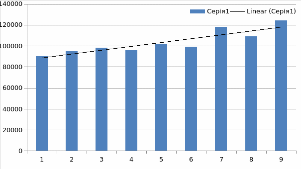
• Least square method determines the values for a and b so that the resulting line is the best-fit line through a set of the historical data.
• After a and b have been determined, the equation can be used to forecast future values.

This method’ overall solution limits possible square errors in solution equations sets. In its sense, the best fit line of best fit minimizes squared residuals summation. The sum of residuals is given by the value differences between observed and availed. Using this method via excel analysis tool yields the following output.

121,861.11 and 116,761.46 sales volume forecasts are recoded for least square and exponential smoothing trends respectively. Despite, the different values obtained, the figures indicate that a high likelihood of increase in sales volume over the coming periods.

Use of control metrics in quality improvement

Use of control charts in improving quality at shuzworld takes into consideration a number of factors. Firstly, the control limits are of essence as they help in determination of the acceptable levels of errors within the production limits (Bisgaard, 1993). The upper and lower control limits assists in achieving this. Processes are always operated within hypothesis that they are in control. Ideally, this hypothesis is not rejected if no changes in process are recoded (Bisgaard, 1993). Often when no changes in processes are recoded though there are changes in signal, Type I errors is considered to have occurred. Often, the actual cause is not found those a reaction to the signal changes are initiated. By convention, most of the variations recoded fall within the control limits and the probability of Type I errors are 0.0027% for shoe sole height samples. However, two points fall beyond the UCL indicating process instability. On basis of the errors beyond the control limits, the process is considered unstable and a reaction must be initiated as though the project is unstable. Likewise for eyeleting fraction defective, two points go far beyond the upper control limit. However, unlike the earlier case, the points are non-consecutive and hence could be considered spontaneous. However, if they present a trend then the process is considered unstable and a reaction is initiated.

References

Brodd, R. (2005). Factors Affecting Production Decisions. Gaithersburg, MD: National Institute of Standards and Technology.

Bisgaard, S. (1993). Statistical Tools for Manufacturing. Manufacturing Review, 6(3), p. 192–200.