Abstract
Correlation and regression analyses were performed to determine the relationship between car retail price and car mileage in the Dubai market. Research data was obtained through random sampling. A questionnaire was given to randomly selected customers in the Dubai car market. MS Excel was used to perform the analyses.
Data Overview
The car retail prices were presented in form of price ranges. The price ranges were coded as follows: 1 – <$3000, 2 – ($3000 to $6000), 3 – ($6001 to $9000), 4 – ($9001 to $12000), 5 – ($12001 to $15000), 6 – ($15001 to $18000), 7 – ($18001 to $21000), 8 – ($21001 to $23000), 9 – ($23001 to $26000), 10 – ($26001 to $29000) and 11 – ($30000 and above). The following mileages were observed: 0, 50000, 100000, 120000, 140000, 150000 and 200000. The car retail prices will be represented by letter X while car mileage will be represented by letter Y.
Measures of Central Tendency and Dispersion
Mean
If there are n values in a data set with values Xi where i = 0, 1, 2, 3, 4…, n, the mean will be expressed as follows:
![]() Or
Or ![]()
Median
The mean can be located by the following formula after arranging the data in order of magnitude:
Median = ½ (n+1) Th figure in a data set. This formula applies to both even and odd data set.
Mode
The most frequent figure in a data set is called the mode. A frequency distribution table showing elements of a data set and the number of times each appears in a data set is used to calculate the mode.
Range
The formula for calculating the range is stated as follows:
Range = Maximum value – Minimum Value
The standard deviation is a measure of the spread of data around the mean. It is calculated as follows:

Where
- σ is the standard deviation
- n is the total frequency of elements in a data set
- xi is the data values
- µ is the mean of the data set
Measures of central tendency (mean, median, and mode) and measures of dispersion (standard deviation and range) are summarized in table 1.
As shown in table 1, the mean, as well as the median and most frequent car retail price ranges, are between zero and $3000. The mean car mileage is about 109,285.7143 miles while the median mileage is 125,000 miles. The standard deviation for the car mileage is 66610.09505 while the range (difference between the minimum and maximum value) is 200000. It is not meant to determine the standard deviation or range for the car retail price ranges.
Correlation and Regression
Correlation is a measure that determines the extent to which two variables’ movements are related. It varies from -1(negative perfect correlation) to +1 (positive perfect correlation). The correlation coefficient is computed using the following formula.
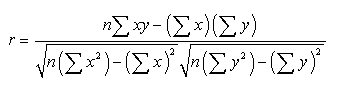
Where r is the correlation coefficient, n is the size of the data, and x and y are the variables.
Correlation analysis produced multiple R-values (correlation coefficient) of about -0.9756. This means that the two variables are highly negatively correlated.
The coefficient of determination (R-square) value of 0.951887 suggests that the regression model was a perfect fit for the data. In other words, approximately 95.19% of the variations in the car retail prices were accounted for by the car mileage data. The other unexplained part of about 5% is explained by other factors not included in the model.
Based on the ANOVA test done, the p-value of F-statistic is less than the level of significance which is 0.05. The rule of thumb is that if the p-value of a statistic is less than the level of significance, then the statistics in a model are jointly significant. F-statistic is a test of the overall significance of the regressors in a model.
Regression analysis is preferred to correlation analysis because it determines the impact of all variables in a model individually and jointly. Correlation analysis only shows the relationship between two variables and cannot analyze a model with more than one regressor. The regression model being determined is stated as follows:
Car price = a + b Mileage +µ. In this case, a is the intercept of the regression equation. It sums up the effects of the variables not included in the model. The slope of the regression model is b and it measures the effects of car mileage on the car retail price in Dubai. Taking x to represent car mileage and y to represent car rental price, the regression equation can be restated as follows:
Y = a + b x + µ
The main aim of conducting regression analysis is to determine the values of parameters a and b. The ordinary least square method (OLS) is used to determine the values of these parameters. The formulas for calculating the parameters by the OLS method are as follows:
b = 
a = ![]()
The results of the regression analysis are summarized in the table below.
Form the results above,
b = 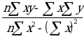 = -1.1E-05 and
a = ![]() = 3.078937
= 3.078937
The regression equation Y = a + b x, therefore, can be stated as follows
Y = 3.078937 – 1.1E-05 x where y is the rental car price and x is the car mileage.
The results of the analysis of variance, P < 0.001 (table 2) mean that the regression model is significant. The regression model can be represented by the following equation: car retail price = 3.078937 – 0.000011 car mileage. The model shows that for every unit increase in mileage, the car retail price range decreases by 0.000011. The p-value of the coefficient of the regression model is 0.000175 which is less than the level of significance 0.05. This means that car mileage is an important determinant of car rental prices.
In conclusion, the car retail price and car mileage in the Dubai car market are negatively correlated. The car retail price would be high when the car mileage is low but low when the car mileage is high. The relationship can be represented by the regression equation, car retail price = 3.078937 – 0.000011 car mileage. The coefficient of determination (R-Squared) was close to 100% meaning that car mileage is a strong determinant of car rental price.
NetWork Analysis
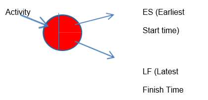
The nods in the diagram represent the following:
The chart is presented as follows:
The following formulas were used in calculating ES, EF, LS, and LF
ES = ES of previous activity + Duration of previous activity
EF = ES for the task + Duration of the task
LS = LF for the task + Duration of the task
LF = LF of the following activity – Duration of the following activity.
Calculations were made possible by the following facts
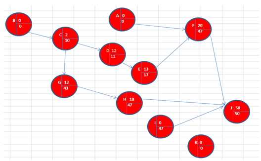
- The first nod in any path has zero ES and LF
- The last node in a path has ES = LF
All activities with negative total float are considered critical events. They include activities A, B, C, D, E, F, J, and K.
The total float for non-critical activities is as follows:
The critical paths are AFJ and BCDEFJ whose total times are 53 weeks and 52 weeks respectively. This means that production cannot start in 48 weeks.