Sales Data
Table 1. Company sales data and forecast sales for 36 months.
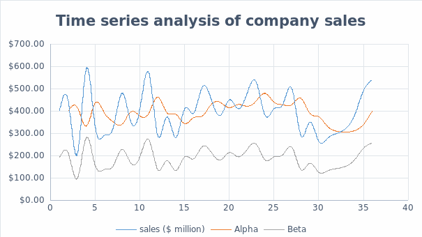
The figure below presents the time series of the company sales for a period of 3 years (36 months).


Discussion
The company sales have fluctuated from time to time, as seen in the figure above. The reason for the variation is not discussed in this paper. However, alpha and beta analyses were employed to predict sales over the proposed period. Although alpha and beta are used in forecasting, they play two different roles, hence the distinct difference in their results (Calle, 2019). Alpha is concerned with smoothing the time series curve by calculating the best coefficient for that particular purpose. On the other hand, beta forecasting is focused on smoothing the trend. Both forecasts use coefficients to achieve the purposes mentioned above. The analysis was carried out with an alpha= 0.4 and beta= 0.475394027.
Based on figure 1 above, the beta forecast is identical to the compare sales except that the two have a huge difference. The difference between the actual sales and the beta forecast sales is 207.991696. Statistically, such a colossal error value could significantly affect the validity of the results obtained. It implies that relying on this forecast strategy is ineffective and could potentially mislead the company in making financial forecasts and extensive budgeting processes.
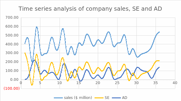
The alpha forecast curve is almost similar to that of the actual company sales. However, the values differ from month to month, which clearly indicates the reliability of the alpha coefficient in forecasting company sales. As seen in the figure above, the alpha curve lags behind the actual sales curve. A rise or decline in the actual sales is followed by a subsequent rise or decline in the alpha forecasts, respectively. The average error in the alpha forecasts is 14.9734236, which is far much smaller than the earlier beta forecast error. The small error value can be attributed to higher levels of accuracy of the alpha forecast. Concerning the MAD and MSE, there is a significant discrepancy in the trends of the results obtained. Both analyses lie below the actual sales, with AD producing the lowest curve. The SE curve is congruent to the actual sales, which gives a good indication of foreseeably accurate predictions. The mean monthly sales were $ 396.4722222, MSE was $111.483, while the MAD was $75.583. The above discussion focused on the alpha and beta analysis, where alpha produced the best forecasts. In the second case, the squared error presents a more accurate prediction than the absolute deviation. The absolute deviation overlooks the potential variations caused by ignoring the negative values that arise from calculations.
With respect to the results obtained, the Alpha forecast is the best approach that the company can use to predict its future sales and financial performance. The results have shown that this approach has a small error value as compared to the beta approach. Besides, the visual presentation of the actual sales and respective forecasts shown in figure 1 is clear evidence of the reliability of the alpha approach. The values of the alpha forecast are almost the same as those of the actual sales, which makes it highly reliable. With reference to Mean absolute deviation (MAD) and mean square error (MSE), MSE is the better choice as it produces close and congruent results to the actual values.
References
Calle, M. Luz. “Statistical analysis of metagenomics data.” Genomics & informatics 17.1 (2019). Web.
