Capital Asset Pricing Model Is Not in the Context of Asset Returns

Introduction

Many years have gone by since the Capital Asset Pricing Model was declared dead but it is still widely used to value assets as well as determine the cost of capital of a company. However, no method has come up as a good substitute. Many researchers and authors have criticized the assumptions behind its construction and, more authors have criticized the assumptions behind its construction and, more importantly, a series of studies has revealed facts that contradict the predictions of the Capital Asset Pricing Model. One of the most disturbing facts is that while the Capital Asset Pricing Model predicts that beta is the only reason why expected returns differ, several studies have shown that other reasons also seem to matter.

This model considers the fluctuations in the returns of assets and it is presented in beta. (Poon and Granger, 2003).

Beta measures assets variability from the market rate of the same industry. The capital asset pricing model assists people to calculate returns of assets. This means when one is provided with the beta of an asset then it is easier to calculate the returns of the asset. (Fischer and Jordan, 2007; Lee, Chen and Rui, 2001).

The Capital Asset Pricing Model

Capital Asset Pricing Model measures the relationship between risk and expected return for each asset for the risk-averse investor. An asset will be expected to provide a return equal to its unavoidable risk. This is simply a risk that cannot be avoided by diversifications. The greater the unavoidable risk of avoided by diversifications. The capital asset pricing model shows the relationship between returns and risk of the asset. The relationship between an asset return and its risk, as measured by beta, will be linear (MacKenzie, 2006).

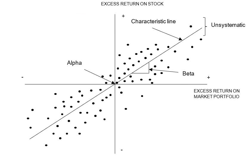
Capital Asset Pricing Model assumes that all assets lie along security line. The figure below shows that the expected return on a risky security is a combination of the risk-free rate plus a premium for risk. This risk premium is necessary to induce risk-averse investors to buy a risky security. The S &p 500 return is used and denoted as RR_m’ the risk free rate is also considered and is recorded as R_f,. This enables one to calculate the risk premium as RR_m’ – R_f. This model does not recognise the fact that the risk is determined by considering the investors preference. Diversification of assets which reduces the value of risk is also not taken into consideration by these models. The investor in only a single security will be expected to both systematic and unsystematic risk but will be rewarded for only the systematic risk that is borne(Merton, 1980).

All assets that are considered are drawn on the same curve and a security line is drawn. The security market line describes the cost of capital for all companies, projects and business opportunities in a given economy at a specific date (Amram, 2002).

As a result, estimating the cost of capital for evaluating a business opportunity is a matter of: (1) estimating the security market line, a general economic relationship that is valid for all companies and that can be obtained from a specialized financial services firm; and (2) estimating the beta coefficient of the business opportunity.

Capital Asset Pricing Model assumes that efficient market hypothesis holds otherwise it will not be successful. The other assumption is that investors are in general agreement about the likely performance and risk of individual securities and that their expectations are based on a common holding period. All investors will perceive the opportunity set of risky securities in the same way and will draw their efficient frontiers in the same place (Akgiray and Booth, 1996).

A security’s expected return should be related to its degree of systematic risk, not to its degree of total risk. If we assume that unsystematic risk is diversified away, the expected rate of return for stock j is

R_jR_j=R_f + (R_mR_f+ (R_mR_j)R_j)βj

Where again R_f is the risk-free rate,RR_m is the expected overall return for the market portfolio, and ββ_j is the beta coefficient for security j as defined earlier. A higher beta means high risk affecting the required rate of return. By the same token, the lower the beta, the lower the risk, the more valuable it becomes, and the lower the expected return required.

Use of Capital Asset Pricing Model

The use of capital asset pricing in the international market requires the consideration of both local and international. The resulting implementation of the Capital Asset Pricing Model depends on which base portfolio is selected. For a company evaluating a foreign investment opportunity, use of its home market portfolio would result in the following version of the Capital Asset Pricing Model:

r_i =r_f +B_ius (r_us – r_f)

where B_ius refers to the project beta when measured relative to the market and r_us is the expected return on the market.

The global capital asset model can be represented as

r_i=r_f + B_ig (r_g – r_f)

where B_ig refers to the project beta when measured relative to the global market and r_g is the expected return on the global market portfolio. the foreign project beta using the global CAPM is computed as follows:

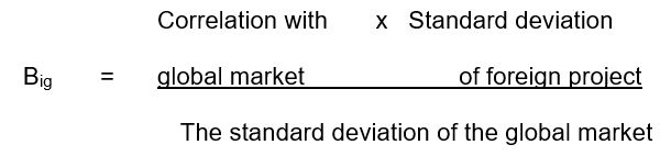
The standard deviation of the global market

The appropriate market portfolio to see in measuring a foreign project’s beta depends on one’s view of world capital markets. More precisely, it depends on whether or not capital markets are globally integrated. If they are, then the world portfolio is the correct choice; if they are not, the correct choice is the home or domestic portfolio. The test of capital market integration depends on whether these assets are priced in a common context; that is, capital markets are integrated to the extent that security prices offer all investors worldwide the same tradeoffs between systematic risk and real expected return. Conversely, if capital markets are segmented from each other, then risk is priced in a domestic context.

Consumption-based models

Some of the models proposed to substitute capital asset pricing models consumption-based models are probably the most general of these models. They start from the idea that investors care for the volatility of their overall consumption. They are not concerned with the volatility of each of their individual assets, provided that they retain a steady rate of consumption. Assets whose payoffs co-vary positively with consumption are not very desirable: they pay off when they are already wealthy and they do badly when they are feeling poor. Only a high expected return might induce investors to buy such assets. On the contrary, assets whose payoff co-varies negatively with consumption are much more desirable and are bought even if they carry a low rate of return: insurance is an extreme case of such an asset. One of the models that likely to replace in Asset Pricing is:

E ((R_i) = R_f + β_i,mλλ_m

Where, E(Ri) = expected return of security I

R_f = risk-free rate

β_i,m = beta factor, the correlation coefficient of security I with m, the discount factor.

This beta factor represent the quantity of risk in security i;

λλ_m = often called the price of risk, is a factor common to all securities that are determined by risk aversion and the volatility of consumption.

Even though not very much used yet in practice, consumption-based models have triggered the ‘equity premium puzzle’ controversy. The equity premiums observed in the past appear to be too high in relation to the volatility of consumption, given the typically assumed attitudes to risk.

Arbitrage pricing theory

The Arbitrage pricing theory model assumes that each security’s return depends partly on events that are unique to that security and partly on pervasive macroeconomic factors. The fact that they respond in similar ways to macroeconomic factors results in the stocks being correlated and one can define a series of macroeconomic factors’ betas. The formula is:

E(R) = R_f + β₁ (R_{factor 1} – R_f) + β₂ (R_factor2 – R_f) + … etc.

Where

β₁ β_2, etc. = various beta coefficients

(R_{factor 1} – R_f) ,(R_factor2 – R_f) etc. = expected risk premiums for the different factors.

The Arbitrage pricing theory does not say what the underlying macroeconomic factors are. Its only prediction is that, because of arbitrage, the relationship between expected returns and the various factor premiums should be linear. Their six factors are:

• Yield spread;
• Interest rate;
• Exchange rate;
• Real Gross National Product;
• change in forecasts of inflation; and
• Stock market return.

Investors should invest in assets that generate positive patterns of stable reinvestment and growth. Arbitrage pricing theory enables investors to price the products of their investments to amass huge profits. An investor should buy cheap assets but with a good return. However, buying cheap and selling high is not as easy as it seems (Brealey, Myers and Marcus, 2007).

This theory holds on to the notion that expected returns from an investment entirely depend on the component of total risks that were involved in it previously (Bodie et al. 2004). Investments with low maintenance costs and debt-to-equity usually contrast this theory. A good investor should ignore the asset pricing theory and invest in the business as long as he or she feels like the investment is worth it. This asset theory also increases the chances of an investment developing maximum debt obligation. This puts such an investment in an awkward position when it comes to weathering economic downturns (Glosten, Ravi and Runkle, 1993).

Factor Models

The capital asset pricing models introduced the idea that risk can be segmented into index-related risk and residual risk. However, very few people would now use a single explanatory variable to model the risk of an asset. They would use instead of more than one variable or factor. These models are sometimes classified into the following categories.

• Fundamental factor models: these models use as factors the company or asset characteristics that, according to experts, explain the differences in asset returns: book-to-price value, market capitalization, recent performance, volatility, etc.
• Macroeconomic factor models: that use macroeconomic variables as factors: industrial production, interest rates, investor confidence, etc.
• Statistical factor models: which rely upon pure statistical analysis to identify the factors.

The models look very much like the Arbitrage pricing theory model above. Some factors that are available in the models that attempt to substitute the Capital asset pricing model are risk factors, measures of profitability, technical factors, and measures of cheapness and liquidity factors. Factor models are very much used for portfolio management but not rally for estimating the cost of capital.

Certain Issues with the Capital Asset Pricing Model

To put across important concepts, Capital Asset Pricing Model has been presented without a number of issues surrounding its usefulness.

Irrelevance is a Capital Asset Pricing Model

It is important to realize that MM’s proof of the proposition that leverage is irrelevant does not depend on the two firms belonging to the same risk class. This assumption was invoked for easier illustration of the arbitrage process. However, equilibrium occurs across securities of different companies on the basis of expected return and risk. If the assumptions of the capital asset pricing model hold, as they would in a perfect capital market, the irrelevance of capital structure can be demonstrated using the Capital Asset Pricing Model.

Consider the expected return and systematic risk of a levered company.

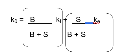
Where, as before, B is the market value of debt, S is the market value of stock, k_i is now the expected return on the firm’s debt, and k_e is the expected return on its stock.

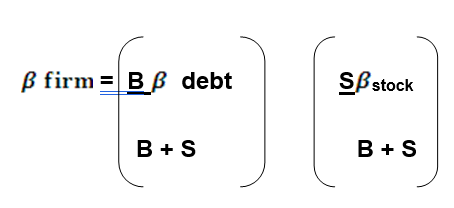
Thus, an increase in the debt-to-equity ratio increases not only the expected retour of a stock but also its beta. With perfect capital markets, both increase proportionally, so that they offset each other with respect to their effect on share price. The increase in return is just sufficient to offset each other with respect to their effect on share price. The increase in return is just sufficient to offset the additional return required by investors for the increment in beta. Therefore, share price being invariant with respect to leverage can be shown in the context of the Capital Asset Pricing Model equilibrating process of risk and expected return.

Maturity of Risk-Free Security

There is agreement that the risk-free rate used in the capital asset pricing model should be a treasury security, which is free of default risk at least in nominal terms. There is disagreement as to the maturity. The capital asset pricing model is a one-period model. As a result, many advocate the use of an interest rate on a short-term government security, like a Treasury bill. Others reason that the purpose of determining a required equity return us to judge whether long-term capital investments are worthwhile (Hagstrom, 1999).

Which maturity is used may make a difference in the required return calculated. This is due to long-term interest rates usually exceeding intermediate-term rates, which, in turn, exceed short-term rates. If the beta of a security is less than 1.0, a higher calculated required equity return will be obtained if a long-term Treasury rate is used. It often is the situation that in public utility rate cases the public rates can be justified, argues for use of the Treasury bill rate. On the other hand, the public utility, which wants a high measured cost, advocates use of a long-term Treasury bond rate. The reason is that most utility stocks have betas significantly less than 1.0(Hull, 1997).

Equity Risk Premium

The expected market, or equity, risk premium, RR_m – R_f, has ranged from 3 to 7 percent in recent years. It tends to be larger when interest rates are low and smaller when they are high. The risk premium is usually affected with the preferences of risk by investors and changes over time. In turn, this is a function of economic and interest-rate cycles. One can easy that it matters whether a short-term, an intermediate-term, or a long-term interest rate is used for the risk-free rate(John, 2002).

For cumulative wealth changes over long sweeps of time, many consider the geometric average to be better. It tells you the amount of wealth you will have at the end, given the annual returns. The arithmetic average best expresses the excess return for a single year. Obviously, it makes a difference which average is used (Theodossiou, 2000).

There is disagreement as to what is the appropriate market risk premium. My preference is ex-ante, beforehand estimate by investment analysts and economists, as opposed to an ex-post, backward-looking return. This allows for a change in the risk premium over time. For now, bear in mind the controversy on which reasonable people differ.

Heterogeneous Expectations, Transaction, and Information Costs

Relaxation of the assumption of homogeneous expectations further complicates the picture. With heterogeneous expectations, a complex blending of expectation wealth and utility preferences of individual investors emerges in the equilibrating process. This complex equilibrating process has been examined by the author elsewhere and will not be presented here. The principal implication is that precise generalizations are not possible. With only moderate heterogeneity in expectations, however, the basic tenets of the capital asset pricing model still hold, and rough estimates of the expected return–risk trade-offs for portfolios and individual securities are possible. Still, the lack of precise description must be recognized(Shapiro, 2002).

Transaction costs also affect market equilibrium. The greater these costs the less investor will undertake transactions to make their portfolios truly efficient. Rather than portfolios being on the efficient set, some may be bands on either side of the efficient set within which portfolios would lie. The greater the transaction costs, the wider the bands might be. Similarly, when securities are not infinitely divisible as is the case in the real world, investors are able to achieve an efficient portfolio only up to the nearest share of stock or the nearest bond. Recall that another assumption of perfect capital markets is that all information about a firm is instantaneously available, free, to all investors. To the extent that there are delays and costs, there will be differing expectations among investors for these reasons alone. The effect here is the same as that for heterogeneous expectations. If it cannot, certain implications of the model do not entirely hold (Scruggs,1998).

Faulty Use of the Market Index

There are problems in the use of any index as a proxy for the overall market portfolio. The “true” market portfolio consists of all assets – stocks, bonds, real estate, and human capital. Roll has analyzed the problem of using the wrong security market line and has categorized errors that can occur. The roll does not suggest that the capital asset pricing model is somehow devoid of meaning but that tests of it are suspect and must be evaluated with caution. Unless the true market portfolio is known and employed, tests of the capital asset pricing model are likely to result in the faulty measurement of security performance. As the proxy market index is only a subset of the true market portfolio, it is unlikely to capture the basis of the underlying market equilibration process. Therefore, the measurement of security performance for various investment strategies will be ambiguous (Poterba, and Summers, 1986).

Fama-French and Beta as a Risk Measure

As we know, the key ingredient in the capital asset pricing model is the use of beta as a measure of risk. Early empirical studies showed beta to have reasonable predictive power as to return, particularly the return on a portfolio of stocks. For sharp downside movements in stock prices, the beta was an effective predictor of riskiness. Increasingly, however, there were challenges, not only for the reasons previously discussed but for others (Fama, 1965).

For one thing, several anomalies were observed which the capital asset pricing model could not explain. Another anomaly is that stocks with low price/earnings and market-to-book-value ratios do better than stocks with ratios. Again this is after the effect of beta is held constant.

In a provocative article, Fama and French (FF) empirically test the relationship between stock returns and market capitalization, market-to-book value, and beta. They found the first two variables to be powerful predictors of average stock returns, having significant negative relationships with average returns. Moreover, when these variables were used first (in a regression), the beta was found to have little explanatory power. Professor Fama, in his wisdom, proclaimed that beta was dead as a variable explaining the returns of any security. Thus, FF launched a powerful attack on the ability of the capital asset pricing model to explain stock returns, suggesting that size and market-to-book value are the appropriate proxies for risk. However, market value is embraced in both variables, and it is market-value changes, together with dividends, which the regressions try to explain. As market value appears in the dependent as well as the independent variables, this is bound to result in explanatory power. A number of critics have attacked FF’s methodology with varying degrees of support for the capital asset pricing model.

Fama-French does not really focus on risk, but rather on realized returns. No theoretical foundation is offered for the findings they discover. Although beta may not be a good indicator of the returns to be realized from investing in stocks, it remains a reasonable measure of risk. To the extent investors are risk-averse, beta gives information as to the underlying minimum return that should be earned. This return may or may not be realized by investors(French and Roll, 1986).

Some Final Observations

The capital asset pricing model is intuitively appealing in that expected return logically follows from the risk security adds to an overall portfolio. Because of its simplicity, the capital asset pricing model is widely used, both in the securities industry and in corporate finance. A workable alternative with superior empirical support has not been advanced. One should recognize that the market equilibration process is complex and that the capital asset pricing model cannot give a precise measurement of the required return for a particular company. Still, the capital asset pricing model trade-off between risk and return is a useful guide for approximating capital costs and thereby allocating capital to investment projects (Angelica, 2005).

However, the model has a number of challenges, extensions of the capital asset pricing model and alternative models are being actively developed (Engle, 1982).

Implications for the valuation of the firm

We have explored some of the foundations of valuation in a market context. Our exploration has not been complete, but we are getting background for a deeper look into the valuation implications of decisions by the individual firm. As we have seen, the value depends not only on the security or firm itself but also on other securities available for investment. By analyzing decisions in relation to their likely effect on expected return and systematic risk, we are able to judge their effect on valuation. According to the presentation so far, unsystematic risk or risk unique to the firm is not important because it can be diversified away. More will be said about this shortly (Chou, 1987).

In keeping with the capital asset pricing model and the separation theorem, we are able to make certain generalizations about the valuation of a firm, without having to determine directly the risk preferences of investors. If management wishes to act in the best interests of the owners, it will attempt to maximize the market value of the stock.the calculated market share price of a stock is usually estimated using the present value of expected future dividends as shown below:

P₀ = 

Where P₀ is the market price per share at time 0, D_t is the expected dividend at the end of period t, and k is the required rate of return. Capital asset pricing model helps organisations trading in the stock market to estimate the required rate of return of a company in any new investments. That rate will be the risk-free rate plus a premium sufficient to compensate for the systematic risk, of course, the greater the risk premium and the return required and the lower the value of the stock, all other things being the same (Christensen and Prabhala, 1998).

Conclusion

The Capital Asset Pricing Model makes conclusions from various assumptions or postulations. Some are crucial or essential to its principle; while others only bring about minor changes if they are fictional. Various attempts have been made to discredit Capital Asset Pricing Model but and no serous model has taken over. The model has the following assumption.

• the model assumes that investors measure Asset risk using the variances of expected returns. All the other measures of risk are insignificant.
• Investors usually wish for more return to less, and they are risk disinclined; that is, they will try to avoid risk if all else is equal.
• Money can be borrowed without any limitation.
• All potential investments are dealt with in the market and are available to everybody, the assets are substantially devisable, and there aren’t limitations on short selling.
• The market is rightly efficient, meaning that each investor gets and understands the same information, then processes it correctly, and trades with no cost. The tax effects of the Capital asset price model are not included when analyzing this case.

To modern researchers and writers’ capital asset pricing model appears like a much-blunted instrument. According to Whitman, planned investment can change at every interest rate. An increase in the expected returns of an asset will produce a shift of the marginal curve towards the left. Whitman claims that British companies continue to demand return rates on the new investments that are much higher, undermining the ability of the industry to re-equip as well as closing the gap of productivity with the compositing.

Reference List

Akgiray, V., & Booth G, 1996. The stable-law model of stock returns. Business Economic Statistics.

Amram, M., 2002. Mapping Corporate Growth Opportunities. Massachusetts: Harvard Business School Press.

Angelica, R., 2005. The asset mix is the key to investment strategy. Massachusetts: Harvard Business School Press.

Brealey, R., Myers, S., & Marcus, A., 2007. Fundamentals of Corporate Finance. New York: McGraw-Hill Irwin.

Bodie, Z., Kane, A, & Marcus, A., 2004. Investments. Boston: McGraw-Hill/Irwin.

Chou, R., 1987. Volatility persistence and stock returns- some empirical evidence using GARCH. Journal of Applied Econometrics, Vol. 3, pp.279-294.

Christensen, B., & Prabhala,N., 1998. The relation between implied and realized volatility, Journal of Financial Economics 50, pp.125–150.

Engle, R., 1982. Autoregressive conditional heteroscedasticity with estimates of the variance of United Kingdom inflation. Econometrica. Vol. 50, No. 4, pp.987-1008.

Fama, E., 1965. The behavior of stock market prices”. Journal of Business. Vol. 38, pp. 34-105.

Fischer, D., & Jordan, R., 2007. Security Analysis and Portfolio Management. New Delhi: Prentice-Hall of India Private Limited.

French, K., & R. Roll, R., 1986. Stock returns variances: the arrival of information and the reaction of traders. Journal of Financial Economics. Vol. 17, pp. 5-26.

Glosten, L., Ravi J., & Runkle, D., 1993. On the Relation between the Expected Value and the Volatility of the Nominal Excess Returns on Stocks, Journal of Finance 48, pp.1791–1801.

Hagstrom, R., 1999.The Warren Buffett Portfolio: Mastering the Power of the Focus Investment Strategy. Hoboken: John Wiley & Sons.

Hull, J., 1997. Options, Futures, and Other Derivatives. Boston: Prentice-Hall.

John, P., 2002. How to Beat the Market Using History’s Best Investment Strategies. Massachusetts: Harvard Business School Press.

Lee, C., Chen, G. & Rui, O., 2001. Stock returns and volatility on China stock markets. Journal of Financial Research, 24, pp.523-543.

MacKenzie, D., 2006. An Engine, Not a Camera: How Financial Models Shape Markets. New York: MIT Press.

Merton, R., 1980. An Intertemporal Capital Asset Pricing Model. Econometrica 41, pp.867–887.

Poon, S., & Granger, C., 2003. Forecasting financial market volatility: A review. Journal of Economic Literature, 41, pp.478–539.

Poterba, J., & L. H. Summers, L., 1986. The persistence of volatility and stock market fluctuations. American Economic Review. Vol. 76, pp.1142-1151.

Scruggs, J., 1998. Resolving the Puzzling Intertemporal Relation between the Market Risk Premium and Conditional Market Variance: A Two-Factor Approach. Journal of Finance 52, pp.575–603.

Shapiro, A., 2002. Foundations of Multinational Financial Management. New York. John Willey & Sons, Inc.

Theodossiou, P., 2000. Skewed generalized error distribution of financial assets and option pricing. Working Paper: School of Business, Rutgers University.