Unemployment Effects on GDP in the US

Introduction

In the contemporary business world, quality management is used to ensure high levels of consistency within firms. This is achieved through practical plans, controls, assurance, and improvements (Dale, Van Der Wiele & Van Iwaarden, 2013: 28). Because quality management does not concentrate on only the quality of goods and services, but also on ways of achieving it, it is important to look at the factors that influence dynamics in the workplace. There is no doubt that quality management is applied to reduce rates of unemployment and inflation across the world. A nation that uses effective approaches to managing quality is exemplified by low rates of unemployment and inflation, but relatively high levels of GDP (Dale et al., 2013: 35). This study has included five variables, which are one dependent and four independent variables. The study has reviewed statistics from the last 34 years (1980 to 2013) regarding the effects of unemployment on GDP per capita in the United States from 1980 to 2013. Statistical process control (SPC) tools are commonly applied to the management of quality in organisations (Dale et al., 2013: 124; Meals, Dressing & Davenport, 2010: 90). In this context, SPC tools have been applied to monitor and control processes, which are key to achieving unique outcomes.

The objective of the study

The focus of this paper is to use SPC tools to improve the quality of organisations. This paper determines if there is any relation between unemployment and other factors, which are tax, inflation, and savings. GDP is indeed influenced by different factors, such as taxation, inflation, and savings. This study aims at identifying the relationship between the dependent variable, which is unemployment, and the independent variables, which are tax, inflation, and savings. Many statistical computations typify it. For example, the regression analysis, scatter plot, and analysis of variance, among other SPC tools, are used.

Hypotheses

The following hypotheses are explored:

1. The null hypothesis is that there has been no relationship between unemployment on the GPD and the inflation on the economy for the past 34 years. On the other hand, the alternative hypothesis that there has been a significant association between the unemployment on GPD and the inflation on the economy in the last 34 years
2. The null hypothesis is that there has been no significant relationship between unemployment on the GPD and taxation on the economy for the past 34 years.
3. On the other hand, the alternative hypothesis is that there has been an important relationship between unemployment on GPD and the taxation on the economy in the last 34 years
4. The null hypothesis is that there has been no significant relationship between unemployment on the GPD and taxation on the economy in the past 34 years. On the other hand, the alternative hypothesis is that there has been a significant relationship between unemployment on GPD and taxation on the economy in the last 34 years.

Literature review

It is worth to state that unemployment is the quality management issue that forms the backbone of this paper. Unemployment is the dependent variable, and it represented by the group of persons that are seeking. However, for people to be included in the variable, they should have been jobless for more than four weeks. All other persons that are laid off by their previous employers are also unemployed. The natural rate of unemployment is sometimes associated with a non-accelerating inflation rate of unemployment.

Labour can be viewed as the rate at which the population is looking for jobs. Labour force participation rate is a critical variable in evaluating growth and unemployment (Hagedorn et al., 2013: 87). It can also be observed as a continued decline in the value of money. Various observations can be made from the definitions. Williams (2012: 2) states that “one price or several prices rising cannot be described as inflation.

Conversely, When there is a general increase in prices or a reduction in the purchasing power of money, then there is inflation. According to Barnes and colleagues (2013: 88), inflation does not affect real output in the end. In the short term, it affects production negatively. Based on their findings, the actual output is not hit in the long term by inflation, but it affects output over the short term. A poor investment plan is as a result of inflation. It leads to price changes and minimises the operations of economic agents (Agrawal & Matsa, 2013: 454). There is a positive link between unemployment and inflation (Hagedorn et al., 2013: 38).

In the United States, the population is responsible for paying annual and quarterly taxes. Taxes that are collected by the government include disposable personal income and personal taxes. Personal taxes are motor vehicle tax, income tax, and personal property taxes. It can be defined as “the income available to persons for spending or saving” (Patton, 2012: 12). Other personal taxes are collected from individuals that own property and are residents of the nation.

There should be a constant saving over some time to achieve equilibrium in the economy (Williams, 2012: 2). Savings rate helps in determining the stock capital of a country. When there is a high rate of saving, a country experiences capital stock, leading to greater output. High saving rates do not necessarily imply less consumption. High saving rates result in capital investment and better economic growth trends. The growth rate of real GDP is higher when personal saving rates increase more than when it declines. It also agrees that GPD leads to improvements in productivity, innovation, and job creation in every field of the economy (Giulietti et al., 2013: 31). There is an observation that the negative impacts of inflation on the economy and the fact that inflation leads to the development of unemployment, leading to the development of slums in the big cities and towns (Williams, 2012: 2).

Data description

The data and information used in this research have been retrieved from the Bureau of Economic Statistics. The data implied many observations. In the 1980s, there was a high rate of unemployment, which has had certain effects on the economy of the nation. Unemployment caused higher poverty rates, showing that the government engaged in endless efforts of trying to cater to the needs of the poor. Besides, with a large portion of the population that contained people that could not support themselves financially, the nation was forced to spend more to ensure that its citizens attained basic needs.

In 1982, the unemployment rate reached a maximum level of 9.7 %. The US has had some poor environmental and social aspects, which have been as a result of unemployment. In 2009, there was an inflation rate of 0.03% that dropped from the previous years. In this case, many people were still dependent on the government for the resources they needed. It can be stated that the inflation rate reduced because there was no longer a high demand for products in the market, which were typified by very high prices. This was due to a large portion of the population was unemployed and created a lack of purchasing power (Williams, 2012: 7). That effectively meant that, as a result of many people being jobless at the time, there was a reduction in the inflation rates. This was shown when the rate of unemployment was very high in 2009.

According to the data, there appears to be an inverse relationship between the labour force and unemployment, which was noticed in 2000. The labour force reached a maximum level of 67.2 million, and employment reached its minimum level of 4%. There is a directly proportional relationship between inflation and taxes, which was noticed in 1980. Saving rates reached a maximum level of 1981, while unemployment was 7.6%. It is very difficult to analyse the budget of the United States and how its economy works for the reason that the nation is a very complex structure, and bearing in mind the size of the country and its population size. In this case, the government has been continuously spending substantial amounts of money to serve the populace (Williams, 2012: 8).

Variables

Unemployment – those without jobs

• Labour force: The active people in the labour market.
• Inflation – An independent variable defined as a continuous or sustained increase in the general price level.
• Tax – An independent variable defined as income available to persons for spending or saving.
• Savings – An independent variable that is defined as the funds that can be amassed within a period, which implies that people can save in the short-term or long-term.

Research and discussion

The following expression shows the regression equation between the dependent and independent variables: Unemployment = 87.6 – 0.218 inflation – 1.24 labor force + 0.084 tax + 0.0177 savings.

The independent variable, inflation, has a p-value of 0.291 that is greater than the significance value of 0.005. Hence, it is not significant and does not contribute to unemployment rates in the nation. This is also analysed based on the R-sq that is 86.1%. This means that the model can account for 46.1% of the errors. Nevertheless, errors are minimal because 53.9% of the errors cannot be accounted for in the analysis.

Unemployment = 87.6 – 0.218 inflation – 1.24 labor force + 0.084 tax+ 0.0177 savings

S = 1.28771 R-Sq = 46.1% R-Sq.(adj) = 38.7%

Analysis of Variance

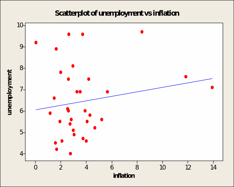
Individual analysis (unemployment vs inflation)

An expression is used to show the regression equation between unemployment and inflation. From the analysis of variance table, the model is not significant since the p-value is 0.317, which is greater than the significance value of 0.005. Thus, inflation does not contribute to unemployment. The scatter plot is on the dependent variable (unemployment) and the independent variable (inflation). This is similar to the view of (Ball, De Roux & Hofstetter, 2013: 400) that showed that taxation does not affect unemployment. The slope of 0.104 showed a positive association between the two variables.

There is no relationship between unemployment and inflation. The value of R is -0.10, showing a weak positive correlation, and at the value of 1.77 is less than 2.048. So, it is accepted at 95%. Regarding the observation, there is no correlation.

R² = (0.031 or 3): This is a proportion or per cent that can be used to state that 3.1 per cent of the variation can be explained by the model.

T value = 1.02 and a p-value of 0.317. The figures imply that there is no significance since the p-value is greater than the significance value of 0.005. Hence, there is no basis to reject the null hypothesis.

The regression equation is

Unemployment = 6.06 + 0.104 inflation

S = 1.64386 R-Sq = 3.1% R-Sq(adj) = 0.1%

Analysis of Variance

Unemployment versus labour force

The expression (R² = 0.416 or 41.6%) shows the regression equation between unemployment and inflation. From the analysis of variance table, the model is not significant since the p-value is 0.317 that is greater than the significance value of 0.005, implying that inflation does not contribute to unemployment. The scatter plot is on the dependent variable (unemployment) and the independent variable (inflation).

The slope of -0.995 shows a negative correlation between the two variables. Unemployment versus inflation shows a no positive relationship with an R² of 0.10 or 10% and R of 0.10, showing a weak positive correlation and at a value of 1.77 is less than 2.048. Thus, it is accepted at 95%. There is no correlation. The findings are supported by other studies (Ball et al., 2013: 400; Mertens & Ravn, 2013: 1220). However, Hagedorn and colleagues (2013: 87) present conflicting results.

R² = (0.416 or 41.6%): This is a proportion or percentage. Thus, 41.6% per cent of the variation can be explained by the model.

t-value = -4.78 and a p-value of 0.000 implies that there is no significance since the p-value is greater than the significance value of 0.005. Regarding the results, it would be prudent to reject the null hypothesis.

Unemployment = 71.9 – 0.995 labor force

S = 1.27597 R-Sq = 41.6% R-Sq(adj) = 39.8%

Analysis of Variance

A scatter plot and a histogram were used because they have significant merits in comparison with other SPC tools. For example, a scatter plot is an instrument that is applied to model data based on the Cartesian coordinates. This implies that values are displayed as a set of data, enabling a reader to form a visual perception of the data. Another merit of the tool is that it is utilised to predict many types of associations that could be evident within a set of data. The greatest advantage of using histograms to represent data is that they provide the probability distribution of data elements, which could be applied to offer insights into a quantitative variable. Another merit is that they could be used to give a rough idea regarding density estimation, which can result in better quality management of various aspects of the economy, such as employment, inflation, and GDP.

Based on the scatter plots, it is clear that there was a strong negative relationship between the primary independent variable (the labour force) and the dependent variable (unemployment). While the additional data from 2010 to 2013 showed a significant change in the Durbin-Watson values (from 1.01 to 0.87), the Durbin Watson values for each showed a positive autocorrelation. Due to the observations, it is worth to state that the results are biased and unreliable. In conclusion, SPC tools used in the research acted as perfect instruments that can provide insights into the issues of unemployment, inflation, and GDP improvements. As illustrated in the study, quality can be significantly improved by using effective SPC tools, which can be applied to compare outcomes within a period.

Recommendations

It is recommended that the government should closely monitor the trends of the various factors of the economy. For example, unemployment rates can be clear signs of how badly the economy is performing. Also, better approaches should be adopted to prevent the negative impacts of inflation on the economy. Finally, the government can use more SPC tools in the future to predict ways of reducing the rates of unemployment and inflation and improving GDP.

References

Agrawal, A, K, & Matsa, DA, 2013. ‘Labor unemployment risk and corporate financing decisions’. Journal of Financial Economics, vol. 108, no. 2, pp. 449-470.

Ball, L, De Roux, N, & Hofstetter, M, 2013. ‘Unemployment in Latin America and the Caribbean’. Open Economies Review, vol. 24, no. 3, pp. 397-424.

Barnes, S, Bouis, R., Briard, P, Dougherty, S, & Eris, M. 2013. The GDP impact of reform: A simple simulation framework, OECD Publishing, Boston, MA.

Dale, BG, Van Der Wiele, T, & Van Iwaarden, J. 2013. Managing quality. John Wiley & Sons, Hoboken, NJ.

Giulietti, C, Guzi, M, Kahanec, M, & Zimmermann, KF. 2013. ‘Unemployment benefits and immigration: evidence from the EU’, International Journal of Manpower, vol. 34, no. 1, pp. 24-38.

Hagedorn, M, Karahan, F, Manovskii, I, & Mitman, K. 2013. Unemployment benefits and unemployment in the great recession: the role of macro effects, National Bureau of Economic Research, New York, NY.

Meals, DW, Dressing, SA, & Davenport, TE. 2010. ‘Lag time in water quality response to best management practices: A review’. Journal of Environmental Quality, vol. 39, no. 1, pp. 85-96.

Mertens, K, & Ravn, MO. 2013, ‘The dynamic effects of personal and corporate income tax changes in the United States. The American Economic Review, vol. 103, no. 4, pp. 1212-1247.

Patton, M, 2012. The key to economic growth: reduce the unemployment rate!. Web.

Williams, JC. 2012. ‘The Federal Reserve’s Unconventional Policies’. FRBSF Economic Letter, vol. 4, no. 34, 1-9.