Present value
Present value is the present of future cash flow. The present value assumes that the dollar today is not equal to the dollar tomorrow therefore it must be adjusted for time and inflation. It is calculated as shown in the case below;
Mr. Peky has been given an opportunity to receive $600 two years from now. The required rate of return for this project is 7%. For us to solve this problem properly, we must calculate how many dollars must be invested at 7% today to have $600 two years from now. In this case, let p be equal to this unknown amount, the problem can be expressed as:
Present Value = Future Value (Present value factor)
PV = An
(1 + k)n
Where K is the cost of capital, n is the number of years, A is future cash flows.
P (1+.07)
Therefore P=$600/1.07=560.75
P, therefore, has a value of $560.75 meaning that the present value of $600 received two years from today is given an opportunity rate of 7%, which is 560.75. Mr. peky has an opportunity to decide whether to receive $560.75 today or $600 two years from now. He can receive either by paying less than 560.75 or decide otherwise.
The present value for mixed streams of cash flows
Where the cash flows are not uniform, to find their present values requires that one should calculate the present values of each future amount by summing up the values.
LMD Company has been offered an opportunity to receive the following mixed stream of cash flows over the next four years.
Year Cash Flow
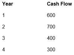
If the firm must earn 10% at minimal on its investments, what is the most it should pay for this opportunity?
Future value
Future value is the value of cash inflows that will be received in the future or paid out in the future. The best example of future value is the interest rate that is paid for a mortgage or for some loan. This amount can be calculated by subjecting the interest to the future value factors. The future value is shown in the case below;
Ruth Mickey wishes to find the present value of $ 2000 that will be received 10 years from now. Ruth’s opportunity rate is 8%. In this problem, we are required to calculate the present value of a future amount. In this case, let Fn be the unknown future value, p be the present value, n to be the years received from now, and I an opportunity rate.
Fn = present value (1 + r)n
Where Fn is the future value, r is the opportunity cost rate and n is numb of years.
Fn = 2000 (1 + 0.08)10= 4317.85
Present value of annuity
The present value of the annuity is the present value of cash flow that is received annually but in an equal amount. The amount should be in a series but equal. In this case, we use the present value factor of the annuity table to calculate the figures. Because of the even cash flows, one figure of the present value of the annuity is used. The following example solves a problem.
The promising company is trying to determine the amount it should pay to purchase a particular annuity. The company requires a minimum return of 10% on all investments; the annuity consists of $900 per year for 7 years. Find the present value of the annuity?
Pn=A(FA4)
Where
Pn=present value of an n year annuity,
A=equals to the amount to be received annually at the end of each year,
FA4= represents the appropriate factor for the present value of the annuity.
Pn =900(4.868)= 4381.2
In solving this problem, one uses a table of present values for an annuity. This table provides values for an annuity of one dollar for specified rates and years. We have tables that contain figures that have simplified the works of students and evaluators. This is because once you find the factor from the table, the present value of the annuity is found by multiplying the factor by the cash flow.
Future value of the annuity
The future value of annuity arises when future cash flows are constant or even. If the company is paying interest with an even amount then the idea of the future value of annuity arises. In this case, the future value of annuity tables is used. The following is an example of the future value of the annuity. If a company receives 10,000 per year for 10 years at a cost of 10%, the future value of this amount will be as follows:
Fn = present value (future value factor of annuity at r% n years)
In our case the present value is 10,000, r is 10% and n is 10 years. From the tables the future value factor of annuity is 15.937. then
Fn = 10,000 (15.937) = 159,370
Bond valuation
Bond valuation is the valuation of bonds. The valuation of bonds is usually done by considering the present value of interest and the terminal amount. The case below shows how bonds are valued.
Mr. James wants to find the value of a 10-year bond with an 8% coupon, paying interest semi-annually, and having a face value of $2000.Assume the market discount rate is 8%.
- Find the present value of the 20 semi-annual interest payments.
Interest per year = 8% x 2000 = $ 160
Interest semi-annually = $160/2 = $ 80 each - Find the present value for interest cash flow.
Find the present value of 20 semi-annual & 80 payments using the assumed market discount rate of 8%. The interest is compounded semi-annually over the 10 years and therefore the present value factor for 20 years and 4% from the table of the present value of an annuity should be used.
Present value factor = 13.590
Present value for interest cash flow = 13.590 x $ 80 = $ 1087.2 - Find the present value of $2000 at maturity.
= $ 2000 x factor for present value of dollar to received at 20 years from now at 8%
= 2000 x 0.456 = $ 912 - Value of the bond
Add the present value for interest cash flow with the present value of maturity value of the bond, gives the value of the bond.
Value of the bond = 1087.2 + 912 = $ 1999.2
The bond value is almost equal to its face value but the small difference is due to rounding error. This is because the market discount rate assumed is equal to the coupon rate. If the market discount rate is higher or less than the coupon rate, the bond value will be different from the face value.
Bonds yield to maturity
Bonds yield to maturity is the actual yield on the bond. The yield will be different from the discount rate if the market value of the bond is different from the par value. This case is shown below. If the market value of a bond is 110 and the par value is 100 with an interest rate of 9%, then the yield to maturity is (9% х 100/110)
Therefore yield to maturity is 8.18%.
Constant growth stock valuation model
A constant growth model is where it is assumed that dividend are received at the constant rate into perpetuity. It is calculated using the following formula;
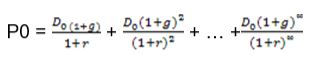
Which can be simplified to P=D1/r-g the following examples show how it should be solved
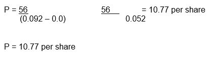
XYZ Company has estimated that its dividends next year will be $ 0.56 per share. On the basis of the past data and certain expectations, the growth rate in dividends is expected to be 4% per year. The rate at which investors capitalize the earnings of similar risk firms within the industry is estimated as 9.2%. Find the intrinsic value of the firm’s stock?
P=D1/Ke-g
Where
P = the price per share of common stock
D1 = the per share dividend expected years
Ke = the equity capitalization rate
G = the expected annual earnings and dividend growth rare.
Substitute
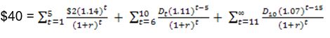
Non-Constant Growth Stock Valuation Model
The non-constant model is where the growth is in phases and is not constant or it can be described as an abnormal growth rate. The best example is when a dividend is growing at 14% for 5 years, then 11% for the next 10 years, and 7% thereafter. The present value will be
P0 = PV(phase 1) + PV(phase2) + … + PV(phase n)
This will be calculated as shown below;
Cost of Capital
The cost of capital is the required rate of return by the company. It is measured as a weighted average of the total cost of raising capital for the company. The cost of debts, the cost of equity, and the costs of preference capital are taken to consideration.
The following example shows the cost of capital.
Assuming the company has a capital structure of the following proportion;
To continue with our illustration, we previously determined that the after-tax cost of debt funds was 6.00 percent and the cost of preferred stock 9.72 percent. If the required return on the market portfolio,Rm is 12 percent, the risk-free rate, Rf’ is 7 percent, and the proxy company beta, adjusted for leverage, is 1.10, then the required return on equity capital is Ke = 7% + (12% – 7%) 1.10 = 12.50%
Therefore, the weighted average required return on investment is
Thus, with the assumptions of this example, 10.27 percent represents the weighted average cost of the component methods of financing where each component is weighted according to market-value proportions.
Capital structure
Capital structure is a composition of the capital of a company. The capital structure consists of equity and debt. The firm can have a debt of a certain percentage on the debt value and equity a certain value. The following example shows a capital structure of a company.
The above is the capital structure of a company.
Capital Budgeting
Capital budgeting is evaluating the project for investment using a certain required rate of return. Capital budgeting involves capital expenditure and expected future cash inflows. It refers to the process of generating, evaluating, selecting, and following up on capital expenditure alternatives. Quite often the capital budgeting process is constrained by the amount of money available for investment. Attention is given to the basic types of projects, the availability f funds, and the approaches to capital budgeting decisions.
Capital budgeting will evaluate the project to determine its viability. An example of capital budgeting is a project which requires an initial investment of 300,000 and the required rate of return is 6% while it will have an annual cash inflow of 70,000 for 7 years. This project will be evaluated using the net present value as follows;
Net present value = present value (present value factor of an annuity of 7 years at 6%) – initial investment.
Net present value = 70,000 (PVIF 6% 7 years) – 300,000
Net present value = 70,000 (5.582) – 300,000 = 90,740
Combination of Capital Structure and Capital Budgeting
In evaluating a capital project a cost of capital is required. The weighted average cost of capital can be calculated from the capital structure and can be used in evaluating a capital project. Take the example of the capital structure in 10 above. The weighted average cost of capital will be
Assume a tax rate of 40%.
Assuming the facts in the case 11 above (The example of capital budgeting is a project which requires an initial investment of 300,000 and the required rate of return is 6% while it will have an annual cash inflow of 70,000 for 7 years) then we shall use the weighted average cost of capital of 7.96% to solve the value of the project.
The project will be evaluated as
Net present value = present value (present value factor of an annuity of 7 years at 8%) – initial investment.
Net present value = 70,000 (PVIF 8% 7 years) – 300,000
Net present value = 70,000 (5.206) – 300,000 = 64.420
Estimating cost of equity and returns
Business organizations are very much dependent on the continuous balance that exists between their monetary inflow and outflow. The cash flow in a business is better determined by the comprehensive way of practically managing the assets of the organization towards the right track that would assure higher returns which is in contrast with the amount of the money they have invested for the business to operate further. There are two elemental factors that are used by business operators to see whether or not they are actually gaining from the business’ operation.
One element is that of the dividend which refers to the payment made by the corporation’s administrators to the shareholders. This money amounting to a certain percentage-part of the overall profit of the corporation within a specific agreed time is considered as a return of value that is supposed to be given to the stockholders who have invested monetary assets as capital for the establishment and a long time foundation of the business.
On the other end, the Rate of Return or the Stock Returns is referred to as the primary amount of monetary returns gained from the business reflected as the business’ profit over an assigned period of time. Considerably, it could be seen that this element is the primary matter that could determine the continuity of the business in the market. This is the reason why adjusting finds and the rate of profit versus loss measurement is given particular attention to by business finance analysts (Hull, 45). It is only through the application of these particular adjustment calculations that the invested amount of money that the business uses as a capital foundation of the organization is better protected for bankruptcy and other monetary imbalances that might happen along the way. True, the real issue to handle herein is the idea of whether or not the stock returns gained by business organizations actually compensate the values that the investors released in support of the continuous growth of the organization. The balance between the dividends released and the profit [returns] gained could be considered as the most efficient backbone of the company that could identify the life of the business. (Fischer and Jordan, 98)
The stock returns would specifically vary depending on the level of control that the administrators have over the dividends that they offer to their stockholders. Skilled traders know that picking the right schedule for pricing an option and releasing the dividends could identify the rate of returns that the organization could receive by the end of each year (MacKenzie, 831)
Making an exceptional identification on how the volatility of assets based on history and current financial status of the business affects the level of gains that the business receives respectively. With the careful assumption of matters through the use of an efficient equation that tends to consider all the elements that are needed to be included as part of the assessment, the Black Scholes Model have been tried and retested over and over and was able to give a considerable result of assumptions that created a great sense of control between the balance that must exist between the dividends released and the stock returns received by a business organization in the international trading market.
At present, this equation for monetary assumptions inquired for business growth is still being developed and restructured for better application and stability. It is very important that the variables used are examined well and that is what the current financial researchers of the said model are doing. At the same time, the application of modern computing systems further makes this measure of connection between dividend and stock returns more efficient and effective for business use. It is expected that after the application of several tries in applying the equation in business financial operations, the process would become more established and more beneficial in the long run (Hull, 87). As of now, the current equation stated within this discussion works well for the values and concerns of business administrators as well as that of their investors. This notes the fact that the current equation provided yields a considerable result that is directly beneficial to international business operators worldwide.
There is a various method of estimating the cost of equity. Some of the methods which are used include the capital asset pricing model, dividend growth model, price-earnings ratio, and other methods which use discounted cash flows.
Since our purpose in finding the firm’s overall cost of capital is to determine the after-tax cost of new funds required for financing projects, attention must be given to the cost of new issues of common stock. A method for finding the current cost of existing common stock was determined in the preceding section, and assuming that new funds are raised in the same proportions as the current capital structure, we need only find the cost of underwriting and selling new issues to find the cost of new issues. It is quite likely that in order to sell a new common stock issue the sale price will have to be below the current market price, thereby reducing the proceeds below the current market price, P. Another factor that may reduce these proceeds is an underwriting fee paid for marketing the new issues.
The cost of new issues of common stock can easily be determined by determining the percentage reduction in the current market price attributable to underpricing and underwriting fees and using the expression for the cost of existing common stock, like, as a starting point. If we let f represent the percentage reduction the current market price expected as a result of underpricing and underwriting charges on a new stock issue, the cost of the new issue, ke, can be expressed as follows;
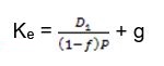
It is quite important that the cost of common stock be adjusted for any under-pricing or underwriting costs in determining the cost of new issues of common stock. The cost of new issues will be greater than the cost of existing issues as long as f in equation 15.8 is greater than zero.
The other model of estimating the cost of capital is the capital asset model. In this model, various items are known. Such items include risk-free rate, market premium, and the beta of a company. In this case, we shall assume the risk-free rate to be 4% and S & P 500 to be 12%. If the company’s beta is assumed to be 1.2, then the cost of equity will be calculated as shown below.
Rs = a + BsRm
Where:
Rs = estimated return on the stock
a = estimated return when the market return is zero
Bs = measure of stock’s sensitivity to the market index
Rm = return on the market index.
Rs = 4% + 1.2(12 – 4)
Rs = 13.6%
Given the assumption of a market model, it is clear that investors can achieve the same diversification as the firm can achieve for them. This point is particularly apparent in the acquisition of a company whose stock is publicly held. In fact, the investor has an advantage in being able to diversify by buying only a few shares of stock, whereas the acquisition for the buying company is much more “lumpy’. Thus, the acquiring firm is unable to do something for investors that they cannot do for themselves at least as efficiently. Therefore, pure diversification by a company through acquisitions is not a thing of value. The acquiring company must be able to affect operating economies, distribution economies, or other synergies if the acquisition is to be a thing of value (Brealey, Myers and Marcus, 226).
This is not to say that an acquisition will not enhance the value of the firm to its shareholders. The prospect f synergism may make a prospective acquisition more attractive to one company than to another, but diversification itself would not be beneficial. Conglomerate mergers for the sole purpose of diversification would be suspect; they would not enhance shareholder wealth. If an acquisition is to be worthwhile, there must be the prospect of synergism. In other words, the acquiring company must be able to affect operating economies, distribution economies, or other things of this sort if the acquisition is to be a thing of value.
References
Brealey, Richard, Myers, Steward, and Marcus Alan. Fundamentals of Corporate Finance. New York: McGraw-Hill Irwin, 2007.
Fischer, Donald, and Jordan Ronald. Security Analysis and Portfolio Management. New Delhi: Prentice-Hall of India Private Limited, 2007.
Hull, John. Options, Futures, and Other Derivatives. Boston: Prentice Hall, 1997.
MacKenzie, Donald. An Engine, not a Camera: How Financial Models Shape Markets. New York: MIT Press, 2006.