How the Theory of Demand and Supply Affects the Supply and Demand of Houses
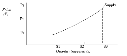
The theory of demand and supply tends to explain the behavior of sellers as well as buyers as far as the price and quantity of goods supplied and purchased is concerned. This model encompasses two scenarios i.e. the quantity supplied and the quantity demanded. It is, in fact, two theories in one i.e. the law of supply and the law of demand. According to the inventor of this theory, Adam Smith, the quantity supplied by the suppliers would be high if the price is high.
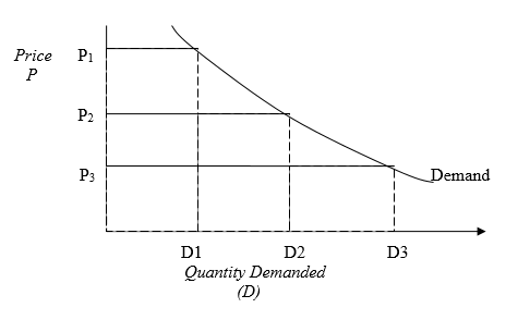
The converse is true; there is a direct proportional relationship between price and quantity supplied. However, there is an inverse relationship between the price and quantity demanded i.e. the higher the price the lower the quantity demanded ceteris paribus. The following diagrams can represent the relationship between the price and quantity.
The Law of Demand
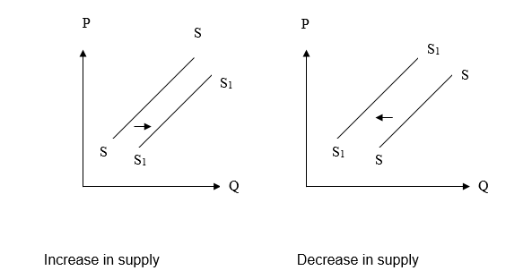
The Law of Supply
Back to his theory of law and demand. He established a point known in economics as the Equilibrium point. This is the point at which the quantity demanded equals the quantity supplied. Diagrammatically, this is represented as below.
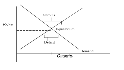
When price falls below equilibrium, demand for the good increases which in turn surpass supply. This creates a shortfall of goods in the market. Suppliers respond to this shortage by increasing the price. The price would therefore be increased until it reaches the equilibrium point. The converse is true; If price gets beyond the equilibrium point, suppliers would supply more of the good (Law of Supply). There would be competition amongst the suppliers to sell the surplus. The end result would be a reduction of prices until the point of equilibrium.
The theorist further came up with the phenomenon of movements and shifts. These occur along both the demand and supply curves.
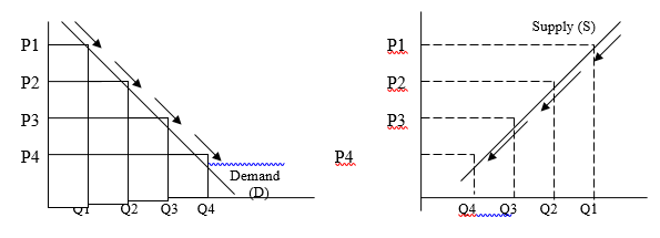
- Demand curve movements: They occur when the quantity demanded changes as a result of price changes only.
- Supply curve movements: These occur when the quantity supplied changes as a result of price changes only.
In both cases, it is assumed that other factors remain constant.
Shifts on the other hand occur when other factors other than price affect demand and supply.
In a normal market place as mentioned above, there is always a supplier and buyer. The buyer creates demand and the supply creates the supply. Therefore, I will define demand and supply in relation to housing
Demand means the willingness and ability of buyers to pay for different services at different fees during a specific period.
Determinants of Demand for houses
There are a number of factors that affect the demand for houses. This includes
- salaries, wages, and benefits offered by the economy.
- charges for rental houses
- government policy on development.
- Information on real estate investments
- performance of financial institutions
- rate of rural-urban migration
- functional characteristics in counties
Changes in Demand, Shifts in demand curves
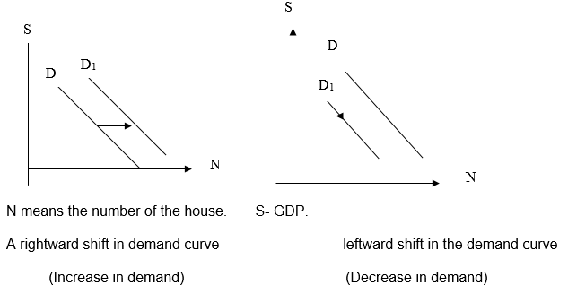
The demand for houses can increase or decrease. The demand for houses increases if more people wanting homes. The demand for houses decreases if the economy is low. The number of houses will increase as the salary increases/economy grows. The demand curve for the houses will shift to the right. If the economic performance comes down then the demand for houses comes down then the demand curve will shift to the left.
Lastly, “if demand and supply change in the same direction, it is possible to know the changes in quantity, but the effect on price is uncertain. E.g. if the price of a complement falls, and also the firm’s technology advances, the demand, and supply curves both shift rightward. As a result, the quantity increases.
And, if supply and demand change in opposite directions, we can always determine the effect on price but the impact on the quantity is ambiguous. For example, if the price of a substitute falls (so that the demand curve shifts leftward) while simultaneously technology advances (which causes the supply curve to shift rightward), the price will definitely fall but the quantity may”
Supply of Houses in an Economy
Supply means the willingness and ability of the public to buy houses at different prices during a specific time.
The quantity of houses supplied is the number of units a good seller is willing and able to produce and offer to sell at a particular price.
The Law of supply
States that as the price of a good rise, the quantity supplied of the good rises, and as the price of a good falls, the quantity supplied of the houses falls.
The law of supply is represented in schedules, graphs, and equations. The supply schedule is the numerical tabulation of the quantity supplied of a house at different prices. The supply curve is the graphical representation of the law of supply.
The Market Supply Curve
An individual supply curve represents the price-quantity combinations for a single seller. The market supply curve represents the price-quantity combinations for all sellers of a particular good. The supply schedule is the numerical tabulation of the quantity supplied of a good at different prices.
Determinants of Supply
- Price of the house itself
- Price of substitute ( rent)
- Price of relevant resources
- Technology
- Number of sellers
- The expectation of future price
- Taxes and subsidies
- Government restrictions
A change in supply versus a change in quantity supplied
A change in supply refers to a shift in the supply curve. A change in quantity supplied refers to a movement along a supply curve.
What factors cause the supply curve to shift?
Prices of relevant resources
Resources are needed to build a house. For example. Wood and cement are needed to produce doors. If the price of wood falls, it becomes less costly to produce doors, and the supply of doors increases
Technology
Technology is defined as the body of skills and knowledge relevant to the use of inputs or resources in production. If there is an advance in technology, the quantity supplied of a good at each price increases. This is because the lower costs increase profitability and therefore provide producers with an incentive to produce more.
Number of sellers
If more sellers begin construct houses, perhaps because of high profits, the supply curve shifts rightward.
Expectations of Future Price
If the price of a house is expected to be higher in the future, producers may hold back some of the houses today. Then, they will have more to sell at a higher future price. Therefore, the current supply curve shifts leftward.
Taxes and subsidies
Some taxes increase per-unit costs.
Subsidies have the opposite effect. If the government subsidizes the construction of one house, the quantity supplied of the house would be greater at each price.
Government Restrictions
Sometimes government acts to reduce the supply
Determinants of Supply of houses
- Information about housing units available and the importance of housing
- Information about the characteristics of houses available and their durability.
- Information about the government policy on housing
- Performance of the economy.
- Policies from various government departments.
Equilibrium
Equilibrium is a situation where supply and demand are in balance. The point where the supply curve and demand curve intersect is the market’s equilibrium. The salary at this point is the equilibrium salary and the number of nurses working for the homes is the equilibrium number of nurses. Equilibrium salary is the relative salary at which the nurses required equals the nurses working.
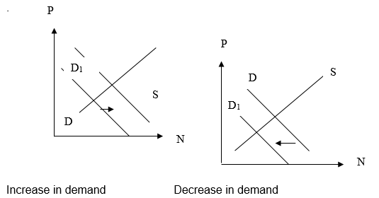
Equilibrium can only change if there is a change in one of the demand or supply conditions or both.
- An increase in demand will raise the Pay for nurses and increase the number of nurses training and working.
- A decrease in demand will lower the price and reduce the number of nurses training and working.
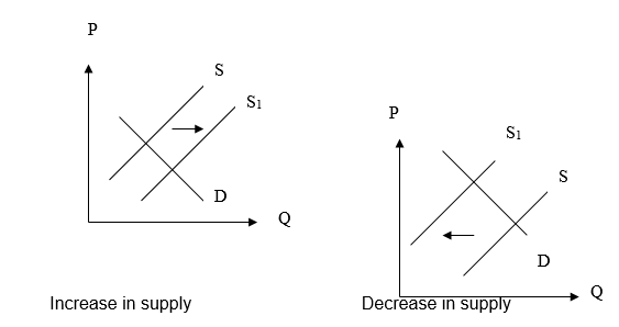
A Change in Supply with demand held constant
- An increase in a number of the number of houses will lower the price
The government through policies will like reduction in interest rate, encouraging mortgages, grants to housing companies
Changes in the price of housing
Using the demand curve for the market and trying to change the prices then the demand for houses can increase or decrease. The demand for houses increases if more price comes down. The demand for houses decreases if prices go up. The demand curve for the houses will shift to the right. If the economic performance comes down then the demand for houses comes down then the demand curve will shift to the left.
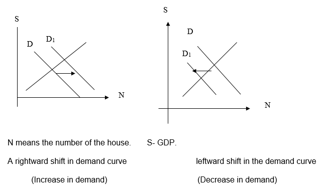
The changes in the price of houses, as shown above, affects the market for other goods and services. Let the subprime be the best example.
the US subprime crisis has already had a global impact on global financial markets and could affect consumer spend worldwide. At first sight, this would seem a disproportionate reaction but banks all over the world are exposed to US debt. Sub-prime lending was lending at higher interest rates as a means of helping American consumers of lower incomes and poorer credit records obtain mortgages. These loans were then sold on, in complex ways, to other institutions including hedge (higher risk higher return) funds. The treatment of sub-prime loans by the banks is likely to have far-reaching effects including, possibly, a slowdown in the US economy and a confidence-linked decline in US consumer spending.
The fact is that US retail sales rose only 0.3% in August 2007 suggesting increasing caution of the crisis ahead. US retail sales are a major driver of economic growth and may be viewed as an early response to a housing slump and financial market turmoil. Over the past 12 months, retail sales rose by 3.9% excluding autos. However, the level of spending did not indicate recession tendencies though analysts expect growth to decline in the near future.
There were modest increases in sales for furniture (0.5%), electronics (0.4%), sporting goods (0.3%), and health care (0.3%) compared with the same month a year ago. Thus, this national economic problem might have a small effect on the health food sector because organic foods are usually priced higher than regular food (Xinhua News Agency, 14 September 2007). This crisis is due to the changes in the prices of houses in the USA.
Most houses have been sold in the market at a lower rate because of the government policy of mortgages. This also affected the purchasing power of the citizens. However, prices varied
From state to state, length of time of the market, and the age and popularity estate for which they were constructed. It had been the experience of the industry for real estate to decline after some time contributing to a downturn in the economy.
From the underlying discussion, it can be concluded that the change in prices of houses affects the purchasing power of the people thus affecting the economy. The example of the subprime crisis as acted as a true example of the effect of change in prices. It means that the increases in prices will lead to an increase in the purchasing power of people. Since the increase in prices is due to demand. Therefore, the government should be able to monitor the change in prices and offer necessary incentives to ensure the economy is not affected.
OPEC
They operate in an oligopolistic competition market. In oligopolistic competition, the market there is a small number of firms unlike in perfect case and the firms are interdependence of firms of each other. The products that are produced by oligopolists may be homogenous.
They can make supernormal profits in the long run or in the short run. However, it can never achieve productive efficiency, as it can never produce at the minimum point of its LRAC. Instead, it always produces at the falling portion of LRAC, when it is making normal profits. Refer to the figure below. Hence, it can never achieve an optimum level of output. The equilibrium price is at OP and equilibrium output is at OQe, which is less than the optimal level. There is excess capacity.
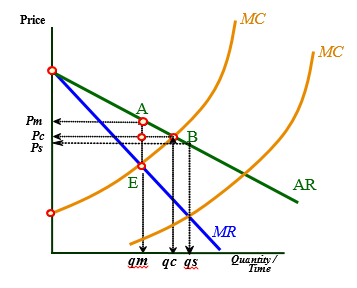
Using the graph above I can deduce that when they increase the price and the demand of the product is in high demand, the economies of the world will slump. It is a price maker and can affect price or output but not both. There are substantial barriers to entry that prevents competition from entering the industry including
- large capital requirements, exceeding the financial resources of potential entrants.
- Legal exclusion of potential competitors
- Absolute cost advantages of the established firm.
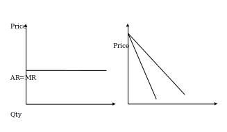
It faces a price inelastic demand curve, as shown in Figure 1(b). AR lies above MR. There is imperfect knowledge due to market failure. Strong barriers are also present.
Comparing OPEC market structure and the ideal market. The differences in price sting will come out openly. Before I compare the perfect and OPEC market I will define it first.
In order, a market to be described as perfect a number of factors must be satisfied. Therefore, I describe perfect competition as a market structure where there a large number of buyers and sellers such that no individual buyer or seller can influence demand, supply, or price and no firm has knowledge of what the other firm is doing. Each firm’s production is minute as compared to total industrial production. All firms sell a homogeneous product that is each firm’s output is indistinguishable from any competitor’s product. Both buyers and sellers are price takers. A price taker is a firm or individual who takes the market price as given. In most markets, households are price takers – they accept the price offered in stores.
There is perfect information that is Firms and consumers know all there is to know about the market – prices, products, and available technology. There is easy entry and exit from the market. If new producers can easily enter and exit the market, existing firms may behave as though there are more firms than there appear to be, because there are more potential competitors.
Perfect competition faces a perfectly price elastic horizontal demand curve, as shown in Figure 1(a). Marginal revenue (MR) equals average revenue (AR) which is also equal to price. Getting an extract from one of the researches done on OPEC and sustainable development.
- price- and standards-lowering competition in the interest of maximizing mass consumption by oil-importing countries by minimizing the internalization of environmental and social costs with consequent destruction of the atmosphere, and ruination of local self-reliance by a cheap-energy transport subsidy to the forces of global economic integration, or
- monopoly restraints on the global overuse of both a basic resource and a basic life–support service of the environment, with automatic protection of local production and self-reliance provided by higher (full cost) energy and transport prices, and with sink rents redistributed to the poor?
Monopoly restraint results not only in conservation and reduced pollution, but also in a price incentive to develop new petroleum-saving, and sink-enhancing, technologies, as well as renewable energy substitutes. Unfortunately, there would also be an incentive to non-petroleum fossil fuels such as coal which would be a very negative effect from the point of view of controlling CO2. Independent national legislation limiting emissions from coal may well be a necessary complement. Ideally, most of us would prefer a genuine international agreement to limit fossil fuel throughput, rather than a monopoly-based restriction imposed as a discipline by a minority of countries only on petroleum. But the Western high consumers, especially the
The US as resoundingly reconfirmed in its recent election, have conclusively demonstrated their inability to accept any restrictions that might reduce their GDP growth rates, even in the likely event that GDP growth has itself become uneconomic, as argued in Part I. The conceptual clarity and moral resources are simply lacking in the leadership of these countries. Perhaps the leadership reflects the citizenry. But perhaps not.
The global corporate “growth forever” ideology is pushed by the corporate-owned media and rehearsed by corporate-financed candidates in quadrennial television-dominated elections. A lack of moral clarity and leadership in mass-consumption societies does not necessarily imply the presence of these virtues in OPEC countries. Do there exist sufficient clarity, morality, restraint, and leadership in the OPEC countries to undertake this fiduciary function of being an efficient collector and an ethical distributor of sink scarcity rents?
As argued above, there is surely an element of self-interest for OPEC, but to gain general support OPEC would have to take on a fiduciary trusteeship role that would go far beyond its interests as a profit-maximizing cartel. But a strong moral position might be just what OPEC needs to gain the legitimacy necessary to increase and solidify its power as a cartel. Could such a plan, put forward by OPEC, provide a stronger power base for the goals that Kyoto tried and failed to institutionalize? Might the WTO and World Bank recognize that sustainable development is a more basic value than free trade, and lend their support?6 I do not know.
Maybe the whole idea is just a utopian speculation. But given the post-Kyoto state of disarray and the paucity of policy suggestions, I do believe that it is worth initiating a discussion of this possibility. If sustainability is to be more than an empty word we have to evolve mechanisms for constraining throughput flows within the environmental source and sink capacities.
Petroleum is the logical place to begin. And OPEC is the major institution in a position to influence the global throughput of petroleum.” (Herman E. Daly 2007) This explains the impact of price increase on the development of the world.
Reasons For Multinationals Operating Abroad- example of British Petroleum
As much as oil companies initially held by governments and their management may try to eliminate the risks associated with internal competition through international operations. The key to successful international operations is the anticipated profits, reduced and control of risks associated with the business. This requires a well-developed for developing a strategic plan. Prudent planning reduces risk.
The major reason for most of these companies going abroad is the increase in cost and availability of stiff competition at home. Therefore, to improve profitability and continual survival of the company international expansion has become necessary. Most oil companies initially owned by governments have gone under especially in third world countries. Forward-looking managers have developed plans to expand to international markets because of the urge to improve profitability and remain in the market, expand a profitable business and acquire new technology, incorporate strategic partners in terms of innovation and technology and achieve economies of scale and spread fixed cost over more business units.
BP
BP adopted a value chain in the international market that has resulted into the maximization of value while maintaining the costs to their minimal levels.
Activities where value has been created and costs reduced include procurement of raw materials, Human Resource Management and Technology development. Other areas include Research & Development, Sales, and Marketing.
In procurement, BP Management has ensured that the raw materials and other supplies are close to their proximity to reduce transportation costs. Oil is refined using high technology while ensuring that their products cannot suffer from impurities and obsolescence hence low obsolescence costs. They incur a significant cost in research and development but this cost is countered by the value generated there from i.e. products that cannot have substitutes.
Value is also added when it comes to outbound logistics. To reduce the distribution costs of oil and other products from the oil depots, the company distributes them in large quantities using tankers while also reducing the number of the distribution channels.
BP tries to reduce the costs associated with recruitment and hiring of staff like for instance doing the exercise online. The benefits/value of the exercise is enhanced by recruiting and hiring staff of high integrity, professionalism and expertise.
Outsourcing
Out sourcing, have many benefits especially when done within the country. Here are some of the benefits:
- Ability to focus on core competencies: By handing over non-core activities to a trusted third party, a company can concentrate on activities central to its value proposition and increase its competitive positioning.
- Faster and higher-quality service and improved efficiency: Vendors’ economies of scale, combined with service level guarantees, translate into increased operational efficiency for a company.
- Access to new skills and technology: Gives a company access to resources not available internally, such as modern, up-to-date technology and skilled human capital.
- Greater flexibility. The flexibility gained helps a company react quickly to changing market conditions, fluctuating demand cycles, and increased competition.
- Staff reallocation. Personnel whose job responsibilities are reduced or eliminated can be reassigned to other, strategic tasks.
- Improved predictability of costs. It provides a company with predictable yearly costs for the management of all.
For multinational, they experience a number of problems while operating in the international market these problems includes: Underestimating the nature international market, most companies assume that their successful services in their country will be equally appealing in the international arena. More often than not, this fails because the service does not fit the market, or the pricing is out of line with the consumers needs.
This can be avoided through following existing clients when expanding into international arena. This strategy result into a win-win situation. This is because the company will have a key resource that will help them in ensuring a successful expansion by providing a solid base for business in the international market. A company without strong home customer base will definitely fail in the international arena. “Regardless of steps you take to get started, you need to be committed for the long term and believe the investment has a reasonable chance of improving both your bottom line and prospects for future growth,” says Karnani.
Operating costs: Operating an office or a any other for of branch in the international market is not like opening a branch in the home country. To avoid this form of costs business leaders need look for strategic partners in the form of alliance, acquisitions, mergers and takeovers. “Financial control problems that lead to theft and loss. In a typical start-up office for a global service expansion, companies will frequently deploy a small team of employees to support existing clients and develop new business. The early financial issues of an expansion office revolve around expenses — such as location costs, travel, meals, housing, and new business development — before gradually shifting to revenue management as business grows” (RMS,2007).Often this companies find open to fraud, outright theft and other malpractices within a small business.
Compliance with statutory requirement: Most communications firms have run into problems complying with laws and regulation of the market they are expanding to. For example, recently a South African subscriber with UK association found them in a tussle with procurement system of a country called Kenya. They were expanding their market share to that region. Apart from this recent case the USA service companies have themselves in the same scenarios. “If a company does not have an internal resource skilled in international tax laws, experts say the next best step is to retain a business services provider that can handle payroll, bookkeeping, compliance and regulatory issues”(RMS,2006).this can be very costly in the long run for the company.
Then to counter those problems they need to outsource for their benefits. Outsourcing per se does not benefit a country as when they could have handled the business without outsourcing. Take an example of Coca Cola outsourcing has brought benefits in to the home country like profits from both sales and transfer costs.
SWOT Analysis
Weaknesses
Nestle Foods faces stiff competition within the industry. Food manufacturing giants dominate the industry. However, because the Nestle Foods has been in the market and the nestle hasn’t touched every household in world, as indicated by the number of factories and countries operating in their competitors have reached. There is a great portion of the consumer base that needs to be tapped especially in most countries in Africa. Even in areas and hot spots where saturation is high, it’s still relatively low compared to the supermarket backbone. It appears that consumers are making a conscious effort away from mass commercialization and inexpensive albeit unhealthy products.
The weakness is that we do not have the learned experience of the giants, but rather than walk in blind, we have research resulting from the actions of our competitors to support our actions. A major threat nestle foods needs to handle is the issue of consumers having now access to variety products from different companies. The industry is financial performance been Fluctuating this is shown from the financial statements.
Strengths
sales IN Dollars BILLIONS Nestle Foods was a viable concept in an industry that had not seen growth as it is happening now. Nestle foods consumers want and are actively engaging in the natural, organic, and fair trade market of goods. Nestle Foods has an advantage as a old competitor because they have been observing growth and development of their industry through infancy indicates that it is time to cash in on an expanding and high-growth market.
Nestle Foods has been objectively considering what works and what does not. They have used R & D in creating models that plays off the faults of the competitors. Nestle Foods identified the need to get down to an individual consumer level, and they employed some aspects of mass customization, bringing the shopping experience away from mega-marts and into the home with basic decisions on the foods. Another advantage is the unique Product Offerings; the company is offering Unique products with strong brand name that has been in the market since in 1866.They have also strong presence in Africa market, strategic position in US and Europe and a commandeering share in the Asian market. They have further embraced the technological know how that is, they are able to produce including organic foods.
Operating in 80 countries with strong staff of 25,000 is another strength that needs to be mentioned. Huge sales have made the company have huge financial base that assists them to be far a head of others in the same industry.
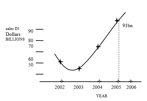
The graph shows that even with the increase in the competition, the nestle foods sales are on the increasing trend.
Opportunities
Enlarging of the Target Market :Nestle company market focuses on customers who are based in development and developing world especially the USA, Europe and Africa. It is expected that both and young old people are the perennial marketing targets of food manufacturing companies from their inception, since everybody is interested in healthy living and wealth is increasing in the world unlike before. In fact, the market for food products has not changed much but with change of wealth, the demand will increase in drastically. Therefore, as people from America and Europe are the historical nestle foods purchasers and users, they will continue to have significant impact on demand for these products therefore forming a key target audience for low and light product producers. Developing countries, on the other hand, have been pushed into taking a more active role in use of this foods purchase in recent years. In general, these youth oriented decisions focus on speed – quick to make, quick to use.
In terms of age, the huge diesel consumers will come from 58 to 80 age brackets. However, youths are a growing market sector for two reasons.
There is increase in demand: The increase in wealth in the world today has led to the increase in demand for food. This is an opportunity for nestle foods to innovate and increase their shares.
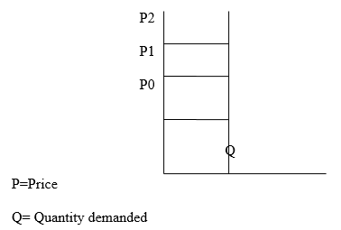
Graph shows that demand for Nestle foods is perfectly inelastic regardless of competition.
Increasing Awareness of People About nestle foods
The competitors are old in the market as well. The modern food companies is a merger of the existing companies and they have really stretched the services they offer. The world is adopting values and objectives of comfort and convenience prevail and these outfits have attempted to cash in on the perks of all-in-one shopping without necessarily offering everything, but specializing and individualizing the experience. Nestle foods can take a hint and develop a strategy that has made them a prime location for food products
Threats
The main threat is direct competition with other multinationals in the industry. They may beat them in quality and service, but not numbers. There is also threat of entry of companies from far east with cheap labor which can cause problems in the industry. This is because there is a trend that most industries are getting the Far East take control of them. This seen in electronic industry.
Additionally, the American market is recessed as a whole. The global trends are shifting to business hotspots outside the US. We are also in the middle of a deadly political war in the Middle East. The financial makeup of our consumers is varied and difficult to gauge but the following assumptions can be made. The ones stuck in the middle, not so much. They are facing a tough job market where outsourcing is a big issue.
Educational and technological standards have shifted drastically and a highly qualified employee 10 years ago is probably going back to school for another degree or specialization in their field. The youth of today are enjoying exposure to the specialty food market and will likely be the carrier of this trend in the future, as other environmental and health concerns will also take precedence in daily life. The threat of an unstable economy right now has indications on multiple levels of strident improvement in the future. The question lies in whether things will get worse, mainly, how bad is the War on Terror going to get and what the US is going to do about reviving the economy.
References
Connor D, and Faille C; (2000); Basic Economic Principles ; Greenwood press.
Robbins L. (2007); The Evolution of Modern economic Theory; Transaction PubBlaug M, Vane H;( 2003) Who’s Who in Economics; Edward Elgar.
Ise J (1925) “The Theory of Value as Applied to Natural Resources”, 1925 (June), American Economic Review.
Herman E. Daly, (1996)Beyond Growth, Boston: Beacon Press.
Herman E. Daly, ( 1991) Steady-State Economics, Washington, D.C. : Island Press.
Salah El Serafy,”The Proper Calculation of Income from Depletable Natural Resources”, in Environmental Accounting for Sustainable Development, edited by Yusuf J. Ahmad, Salah El Serafy, and Ernst Lutz, Washington D.C., World Bank, 1989.
Salah El Serafy, “The Environment as Capital” in R.Costanza, ed., Ecological Economics (The Science and Management of Sustainability), New York: Columbia University Press, 1991.
Salah El Serafy, “Green Accounting and Economic Policy”, in Ecological Economics, 1997.
Roefie Hueting, New Scarcity and Economic Growth (More Welfare through Less Production?), Amsterdam: North Holland Publishing Co., 1980.
Roefie Hueting “OPEC and the Global Energy Balance: Towards a Sustainable Energy Future”, 2001, Vienna, Austria.
Herman E. Daly ;(2007) Sustainable Development and OPEC:School of Public Affairs;University of Maryland.
