The Capital Asset Pricing Model
The Capital Asset Pricing Model (CAPM) specifies the relationship between the risk and the required rate of return on assets when they are held in well-diversified portfolios. Basic assumptions of CAPM would include factors such as investors would be rational and they would choose among alternative portfolios based on each portfolio’s expected return and standard deviation. Investors are usually risk-averse implying that they maximize the utility of end-of-period wealth. In this sense, CAPM is a single period model. Investors have homogeneous expectations with regard to asset return. There exist a risk-free asset and all investors can borrow and lend at this rate meaning that all assets are marketable and divisible. The capital market is efficient and perfect (Wesalo, 2001).
The CAPM formula is given as follows:
Ri = RF + [E (RM – RF)] b
Where:
- Ri is the required return of security
- IRF is the risk-free rate of return
- E (RM) is the expected market rate of return
- b is the Beta.
Note: bi = Cov(im)
____
δ2m
Where
- Cov (im) is the covariance between an asset (i) and the market return.
- (δ2m) is the variance of the market return.
If we graph bi and E(Ri), then we can observe the following relationship
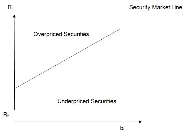
All accurately priced assets will lie on the security market line. Any security that is not found in this line would be either overpriced or underpriced. The security market line, therefore, shows the pricing of all assets if the market were at equilibrium. It is a measure of the required rate of return if the investor were to undertake a certain amount of risk (Hubbard, 2007).
Limitations of CAPM
CAPM has several weaknesses. It is usually based on some unrealistic assumptions. It claims risk-free assets exist, which is not possible in reality. It also believes that all assets are divisible and marketable. In reality, human capital is not divisible. The model believes in homogeneous expectations as regards the expected returns, which cannot be the case in a real-life situation. The assumption that asset returns are normally distributed is misplaced. Another weakness is that CAPM is a single-period model. It looks at the end of the year return only. Moreover, CAPM cannot be empirically tested because we cannot test investors’ expectations. Finally, CAPM assumes that a required rate of return on securities is based on only one factor that is, the stock market—beta. However, other factors such as relative sensitivity to inflation and dividend payout may influence a security’s return as compared to those of other securities.
Arbitrage Pricing Theory (APT)
Formulated by Ross in 1976, the Arbitrage Pricing Theory (APT) offers a testable alternative to the capital market-pricing model (CAPM). This model was formulated to counter the weaknesses of the Capital Assets Pricing Model, which had certain unrealistic assumptions. The main difference between CAPM and APT is that CAPM assumes that security rates of returns will be linearly related to a single common factor that is, the rate of return on the market portfolio. The APT is based on similar intuition but is much more general as compared to CAPM.
APT assumes that, in equilibrium, the return on an arbitrage portfolio that is, the one with zero investment and zero systematic risk, is zero. If this return were positive then it would be eliminated immediately through the process of arbitrage trading to improve the expected returns. Ross in 1976 demonstrated that when no further arbitrage opportunities exist, the expected return (E (Ri) can be shown as follows:
E(Ri)=Rf + β1(R1-Rf)+β2(R2 -Rf)+——–+ βn(Rn-Rf)+έi
Where:
- E (Ri) is the expected return on the security
- Rf is the risk-free rate
- Βi is the sensitivity to changes in factor i
- έi is a random error term.
APT and CAPM compared
The Arbitrage Pricing Theory (APT) is much more robust than the capital asset pricing model for several reasons, one being APT makes no assumptions about the empirical distribution of asset returns. CAPM assumes a normal distribution. Again, the APT makes no strong assumption about individuals’ utility functions (at least nothing stronger than greed and risk aversion). As it can be observed, APT allows the equilibrium returns of an asset to be dependent on many factors, not just one (the beta). The APT yields a statement about the relative pricing of any subset of assets hence one need not measure the entire universe of assets in order to test the theory. There is no special role for the market portfolio in the APT, whereas the CAPM requires that the market portfolio be efficient. Finally, the APT is easily extended to a multi-period framework, as opposed to CAPM.
Limitations of APT
APT does not identify the relevant factors that influence returns nor does it indicate how many factors should appear in the model. Important factors are inflation, industrial production, the spread between low and high-grade bonds and the term structure of interest rates.
Dividend Growth Model
This model was formed on the basic assumption that future string of dividend will have a constant growth rate. This model is therefore used to calculate the basic value of an asset. If the dividend per share paid out in one year is expected to grow in perpetuity at a constant rate of for instance r%, then the intrinsic value of this asset is:
Stock value (V) =DPS
____
r-g
Where:
- DPS = Expected dividend per share, one year from now.
- r = investors required rate of return
- g = dividends growth rate in perpetuity
Limitations of Dividend Growth Model
It assumes that dividend payout will grow at a constant rate in perpetuity, which is not the case in the real investment world. Constant dividend growth might only be realistic in already well-established companies. There are normally many uncertainties like the company making losses resulting in non-payment of dividends, the company going into liquidation, non-declaration of dividends and non-systematic declaration of dividends, are some of the factors that are not considered by the Dividends Growth Model.
Since APT makes fewer assumptions than CAPM and more realistic assumptions than the Dividends Pricing Model, it may be applicable. However, the model does not state the relevant factors. APT has however shown that the security returns are sensitive to the following factors: unanticipated inflation, changes in the expected level of industrial production, changes in the risk premium on bonds, and unanticipated changes in the term structure of interest rates (Shan, McGuin, & Waller, 2007).
In my personal opinion, the use of the Arbitrage Pricing Technique would be recommended because of the previously mentioned reasons. Should an investor decide to use this model then the acceptance rule of the same should be applied. The rule states that if the investment were giving anything lower then that project would not be viable. Furthermore, if the rate of return is lower than the accepted rate of return then the investment is not viable and should be rejected. In a situation where the rate of return is equal to the minimum acceptable rate of return then the investor needs to be indifferent and should consider other factors as whether to invest or not. Such factors could include the time within which they get their return, amongst other factors (Stan, 2009).
Computation of cost of capital using the CAPM
Sony Corporation
E(rj ) = RRF + b(RM – RRF
= 0.20% +1.98(6.83%-0.20%)
= 13.3274%
= 13.33%
McDonalds Corporation
E(rj ) = RRF + b(RM – RRF)
= 0.20% +0.29(2.94%-0.20%)
= 0.9946%
= 0.99%
Sony Corporation has a higher cost of capital of 13.33% compared to McDonalds Corporation’s 0.99%. This is because Sony Corporation has a higher beta and a high rate of return (Anand, 2007). In relation to the entire market, Beta is the amount of unpredictability or systematic risk of an asset or portfolio. Expected return on the Market portfolio is what that security can pay in returns. These two factors affect the rate of return on a portfolio. The higher the two factors, the higher the rate of return. This is because these factors determine the rate of return of a security. In the above case, Sony Corporation has a beta and expected rate of return of 1.98 and 6.83% respectively, as compared to McDonalds Corporation’s 0.29 and 2.94 for beta and rate of return respectively. If any or both of these factors are high, the investor is advised to accept a higher rate of return.
References
Anand, S. (2007). Optimizing Corporate Portfolio Management: Aligning Investment Proposals with Organizational Strategy. New York, NY: Wiley.
Hubbard, D. (2007). How to Measure Anything: Finding the Value of Intangibles in Business. New York, NY: John Wiley & Sons.
Shan, R., McGuin, P., & Waller, J. (2007). Project Portfolio Management: Leading the Corporate Vision. Basingstoke: Palgrave Macmillan.
Stan, R. (2009). Louisiana Joins Build America Bond Parade with $121 Million. Wall Street Journal, 3(1).
Wesalo, T. (2001). The Fundamentals of Municipal Bonds: The Bond Market Association. New York, NY: John Wiley and Sons.