Coats Group’s Financial Markets and Investment Analysis

About the company

Coats Group is a global leader in the industrial thread and consumer textile crafts business. Also, it comes second after YKK Group in the production of zips and fasteners. Currently, the company has a presence in 50 countries that are located on six continents. In addition, it has a sales presence in more than 100 countries. Besides, it has employed about 19,000 people in its outlets (Coats Group PLC 2016a; Coats Group PLC 2016b). Appendix three shows the ratios for the company between the year 2013 and 2015. The profitability level of the company deteriorated during the period. This can be seen in the decline of values of the three ratios.

Further, in 2015, the values of the ratios were negative. This shows that the expenses exceeded revenue generated (Yahoo Finance 2016). This indicates that the company is inefficient in handling expenses and revenue. The company had a high liquidity level. This shows that the company has the ability to pay immediate obligations promptly. However, extremely high ratios can be an indication that the company is concealing liquidity problems. The proportion of debt in the capital structure increased as indicated by the growth of debt to equity ratio over the period. The increase partly explains why the return on equity dropped.

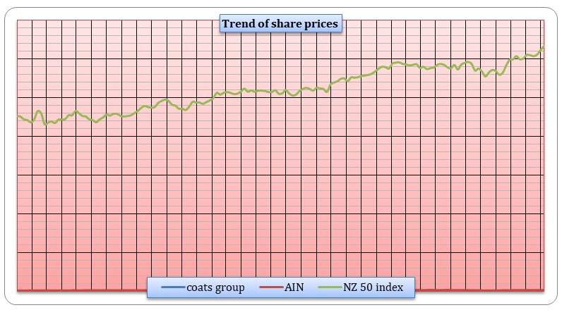
The interest coverage ratio increased over the period. This implies that the company is solvent. The efficiency of the company fluctuated during the period as indicated by the asset management ratios. The values deteriorated in 2014 and later improved in 2015 (Coats Group PLC 2016c). The graph presented below shows a comparison of the weekly share prices for the company, market index and for a competitor. The data for the share prices is presented in appendix 4.

Yield curve

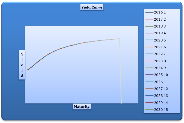
The data for spot rate and maturity New Zealand is presented in appendix 1. The yield curve for New Zealand is presented below.

Discussion

The yield curve presented above shows the relationship between the spot rates for the risk free discount rates as at 31^st December 2015 and maturity. The curve is sloping upwards. It is worth mentioning that the shape of the yield curve differs across various countries and it is determined by the supply and demand of funds at various maturity levels in a country’s debt market. In curve above, long term debts have higher yield as compared to short term bonds. This is can be explained by the fact that the high risks that are associated with time (Brigham & Ehrhardt 2013).

There are a number of reasons that can explain the shape of the New Zealand yield curve above. The first reason is that the higher yields for long term debt are supposed to compensate the investors for the low liquidity that they will experience. Further, investors are exposed to high risk of loss if they need to sell the debt before its maturity. This can be attributed to the fact that long term debt is more responsive to changes in market interest. This explanation is consistent with the liquidity preference theory. Apart from the forces of demand and supply, there are a number of other factors that affect the yield curve of a country (Choudhry 2011).

An example is the interest rate expectation. For instance, if investors anticipate that the county will experience a recession, then the yields for short term debts will be higher than those of long term debt. This creates the downward sloping yield curve. However, if investors anticipate that the economy will experience a boom in the future, then the long term interest rate will be higher than the short term rates. This leads to the upward sloping yield curves. This is consistent with the expectation theory. Apart from expectation theory, inflation also has a significant impact on the shape of the yield curve. In the case of New Zealand, the yield curve is rising. This can be explained by the fisher effect which outlines that the rising yield curve can be explained by the fact that high level of inflation are expected in the future. On the other hand, if inflation is expected to drop in the future, then the yield curve is likely to slope downwards.

A small hump can be observed on the yield curve presented above. This hump can be explained by the preferred habitat theory. Based on this theory, the market is segregated in such a way that various market participants have preference for different maturities. Concentration can be observed in debts that have short and long maturities. The hump is attributed to the fact that there is low demand for medium term maturities. Further, the difference between the short run and long run rates also affects the shape of the yield curve. If the gap between the short term and long term rates is high, then the slope of the yield curve is likely to be steep. Otherwise, if the gap between the rates is small, then it may result in a flat yield curve.

Market risk premium

The concept of market risk premium is vital because investors use it in the capital asset pricing model. It is measured by the difference between the expected return on the market portfolio and the risk free rate of return (Damodaran 2010).

Market risk premium = Rm – rf

The historical market risk premium is similar for all investors, because the value is based on past occurrences. It shows the historical difference between the return of the market and treasury bonds. Finally, the expected market risk premium is the difference between the return of the market over treasury bonds. Countries always provide an equity risk premium over the long term debt instruments. Besides, studies have always indicated that historical results are unbiased estimate of the expected future long-term equity risk premium. The long-term expected future equity risk premium for New Zealand is estimated to be 4% (The Treasury 2016). This value is arrived at after taking into account the past record of the market return, reported earnings, dividend, forward looking information through surveys and expectation of future earnings (Damodaran 2012a).

As mentioned above, the historical market risk premium is the same for all investors. However, the market risk of all assets differs. Despite this contrast, the concept of market risk premium is still relevant under the current market conditions. It has clear implications for all players in the market. For instance, if an entity wants to raise capital, then it must use the market risk premium to estimate the cost of capital (Damodaran 2012b). On the other hand, investors drive the market risk premium through their willingness to assume risk and invest in risky securities. Therefore, market risk premium aids in matching up capital and other factors of production. Besides, it creates order in the financial markets by improving trust in the financial markets. Thus, market risk premium is a key element of every risk and return model (Elton & Brown 2007).

Estimation of beta using the market model

Market model

The model states that the return on a stock relies on the return on the market portfolio and the degree of sensitivity of the stock. The responsiveness of the stock are measured using the beta. Also, the return depends on the conditions that are specific to the firm. This model is similar to the single index model except for the fact that the assumption of zero covariance (cov (eiej) = 0) is not made (Lee, Lee & Lee 2009). It is worth mentioning that the total risk of a stock is the sum of unsystematic and systematic risk. This can be expressed in an equation which states that the return on any asset can be expressed as a linear function of the market return and random error. This linear relationship is known as the market model and it is presented below.

R_i = α_i + βiR_m + e_i

The use of the ordinary least squares method to carry out a regression analysis reduces the error term to zero. This reduces the equation to;

R_i = α_i + βiR_m

The regression equation will model the relationship between the return of the risky asset and the return of the market portfolio. The resulting regression line is also called a characteristic line (Mandura 2007). The outcome of the regression line will give results for both systematic and unsystematic risk. The intercept of the regression line (α_i) is the alpha coefficient of the stock. The slope of the regression line measures the responsiveness of the return of the individual assets to the market portfolio.

Regression results

The data that is used for the regression analysis and the result are presented in appendix 2.

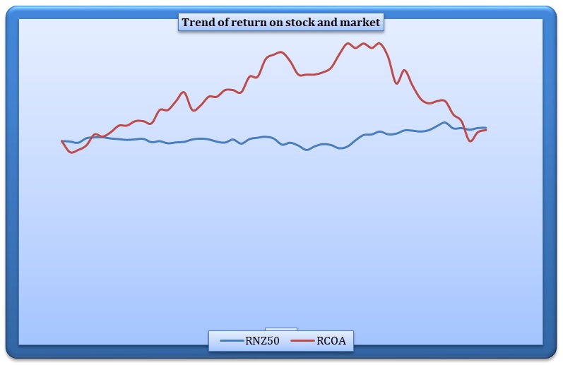
The dependent variables are the returns on the stock of Coats Group PLC while the independent variable is the return on the prices of the New Zealand 50 index. The results of ANOVA show that the value of F-significance is greater than the value of the alpha. This implies that the overall regression line is not valid. Also, the coefficient of the slope of the regression line is not statistically significant because the P-value of the slope is greater than the value of alpha (0.05). The coefficient of determination (R-square) is 4.78%. The values are quite low and it implies that the model used does not fit the data well (Baltagi 2011). Therefore, the beta will not be used in the analysis. Therefore, the industry values will be used. The beta for the apparel industry is 1.06.

Capital asset pricing model (CAPM)

CAPM return = risk free rate of return + beta * market risk premium

The risk free rate of return for the current year (2016) = 2.57%

Beta = 1.06

Market risk premium = 4%

Return = 2.57% + 1.06 * 4% = 6.81%

Actual return

Share prices as at 1^st February 2015 = NZD0.46

1^st February 2016 = NZD0.49

Dividend = 0 = (0.49 – 0.46) / 0.46 =0.06522 = 6.52%

Based on the calculations above, the return estimated using the CAPM model is greater than the actual return. This shows that the security is undervalued and an investor should buy the stock of Coats Group PLC because the share prices are likely to rise. Thus, an investor will gain the future by holding the shares (Bodie, Kane & Markus 2012).

Assumption and critique of the model

The discussion above indicates that an investor should purchase the shares of Coats Group PLC (NZ). This is based on the fact that the stock is currently undervalued. This decision is based on the assumption that the undervaluation of the shares does not imply that the company is facing serious financial management issues. Besides, it is also assumed that there will be no significant changes in the values that are used in the model. This will ensure that the current valuation will not change by a large margin in the future. However, the investor should continue to monitor the financial performance of the company. This is based on the fact that the performance deteriorated over the past three years. The monitoring will ensure that the trend will not persist in the future.

The CAPM model that is used in the valuation above has a number of shortcomings. The first drawback is that the risk free rate of return that is used in the model changes on a daily basis thus creating volatility in the model. Secondly, the model cannot be used effectively in scenarios where the market return is negative. Besides, future market return may not follow the historical trend as outlined in the efficient market hypothesis and the random walk hypothesis. Thirdly, the model is based on the assumption that an investor can borrow and lend at the risk free rate of return.

This does not seem to be practical in real life. The model also assumes that investors have an absolute free access to all available information. It also assumes that investors have an identical expectation of risk and return. Finally, the model is based on the assumption that investors are rational when making investing decisions. Therefore, despite its widespread use, the model is highly criticized for its unrealistic assumptions.

References

Baltagi, G 2011. Econometrics, Springer, New York.

Bodie, Z, Kane, A & Markus, A 2012. Investments, McGraw Hill Publishing Company, USA.

Brigham, E & Ehrhardt, M 2013. Financial management theory and practice, Cengage Learning, Boston.

Choudhry, M 2011. Analyzing and interpreting the yield curve, John Wiley & Sons, New York.

Coats Group PLC 2016a. About us. Web.

Coats Group PLC 2016b. Change of name. Web.

Coats Group PLC 2016c, Fact Sheet. Web.

Damodaran, A. 2010. Applied corporate finance, John Wiley & Sons, New York.

Damodaran, A. 2012a. Equity risk premium (ERP): determinants, estimation, and implications – the 2012 Edition. Web.

Damodaran, A. 2012b. Investment valuation: tools and techniques for determining the value of any asset, university edition, John Wiley & Sons, New York.

Elton, G & Brown, G. 2007. Modern portfolio theory and investment analysis, John Wiley & Sons Ltd, USA.

Lee, A, Lee, J & Lee, C. 2009. Financial analysis, planning & forecasting: theory and application, World Scientific Publishers, New York.

Mandura, J. 2007. International financial management, Cengage Learning, Boston.

The Treasury.2016. The market equity risk premium. Web.

Yahoo Finance. 2016. Coats group PLC (COA.NZ). Web.

Appendices

Appendix 1

NZ Risk-free Discount Rates.

Appendix 2

Estimation of beta.

Appendix 3 – Ratios

Appendix 4

Share prices.