A Preliminary Time Series Test of Growth Models

This reports on an effort to test the exogenous and endogenous theories of economic growth employing OLS regression on a sample of time series data from the Penn World database. The trial run was only partially successful owing to the limited variables in the dataset and because preliminary test runs precluded log transformation of the Y variable and iterative runs on the lagged treatment of the independent variables for labor pool and savings/investment.

The oil shocks in the last three decades of the 20th century and the current recession that commenced in America in the latter half of 2007 reinforced old lessons and drove home new, puzzling ones. First is the necessity for sustained economic growth to afford national populations’ continuously improving standards of living. Secondly, beginning with the geopolitical aftermath of the 1973 Yom Kippur War – the OPEC crude embargo and the first of many ‘market-oriented oil price shocks – Butzin (1997) notes how the most industrialized countries – the UK, the United States, Japan, Germany, and France – experienced long periods of sluggish performance while the newly industrializing nations of East Asia went from strength to strength. In a contemporary world, thirdly, of inextricable dependencies based on trade and financial flows, it stands to reason that the collapse of the home mortgage bubble in the U.S.A. spilled over across the seas to trigger varying levels of decline in such diverse trading partners like the UK, Ireland, France, Germany, India, Japan, Korea, Malaysia, and Singapore. But some factor or other enabled the Philippines, the Republic of China, and mainland China, all just as dependent on trans-Pacific trade, to keep their heads above water.

These factors, among others, have restarted the debates about sources of economic growth and the theories of convergence that neo-classical economics had postulated for long-run stability.

In particular, more attention has been paid to deriving support for the exogenous and endogenous models of economic growth. In part, these continuing investigations were required by the fact that the Solow model was initially fitted to U.S. economic growth rates through the middle of the century.

Having been put forward earlier, the Solow growth model attracted more efforts at empirical testing. Solow (1956) had thought to augment the Harrod-Domar model on savings rate as the engine of economic growth by proposing the importance of investment.

A second factor that enters the Solow framework is the stock of labor. Population growth is needed to keep the gross domestic product (GDP) rising. But the relationship is not directly proportional after a certain point is reached because, Solow argues, incremental deployment of capital (see Figure 1 overleaf) is subject to diminishing returns of production. Since the population is external to the interplay of microeconomic functions like production, cost, price, and consumption, the Solow model became the archetype of ‘exogenous’ analyses of national growth.

The third facet of the Solow proposition is that the growth rate of nations is inversely proportional to the status of per-capita gross national income. The least-developed and developing economies are bound to demonstrate higher growth rates until the community of nations arrives at a point of convergence between high- and low-income countries. In Figure 1, this is shown as the midpoint of the straight line production function (n + d)k. At point A, the “steady-state”, there is equilibrium and production rises so long as the population continues to rise (or the nation admits more immigrants.

Output increases with labor pool growth when the savings rate is high enough to provide enough capital stock to accommodate a rising population (n). In the model, this is where the orange production curve rises sharply from point y₁ to point y₀.

Unless new, heightened savings can be deployed (or earned from foreign trade surpluses or sourced from borrowings), capital depreciates and no longer grows as rapidly as it used to. It declines on a per-capita basis.

Endogenous theories, on the other hand, better explain the experience of divergent economic growth among countries. This set of theories assume that a nation can leverage technological innovation only if it has a steadily rising pool of human and physical capital.

At the core, endogenous growth theories explain the role of innovation as making a particular sector more productive or birthing new sectors that increase productivity for the economy as a whole. This framework originates from explicit analysis of innovation as outcomes of profit-seeking activities’¹ showing the relationship between profit maximization and endogenous growth, which possibly explains the reasons for different trends in the rate of growth. Endogenous growth rate theories also explain the role that investment in education plays in paving the way for trained manpower and therefore energizing national growth².

Endogenous models include the ‘increasing returns to scale’ proposition put forward by Paul Romer and the ‘human capital theory of Robert Lucas. In contrast to the exogenous theorists, Romer (1986) argues that country growth rates can continue indefinitely (i.e. diminishing returns do not necessarily apply) and that large economies will perennially outperform less-developed nations. More importantly, he insists that production cannot take place efficiently without knowledge and that the latter must have positive effects.

Romer assumes, first of all, that there is an exogenous rise in the knowledge time T > 0. Equilibrium trajectory rises rapidly up to time T. At the equilibrium point, the economy leverages a rise in capital stock to rise to CE. However, the growth path for t remains autonomous and shows positive marginal growth.

The y axis, λ, denotes the rate of growth, K on the x-axis represents capital stock, and the middle curve, λ=0, represents the growth path when there is no exogenous introduction of knowledge. In other words, there has been virtually no investment in education or R&D.

The author embarked on an empirical inquiry of both the convergence and divergence theories of economic growth employing time series analysis of a sample of countries in the Penn World Tables database for the period 1950 to 2004: Afghanistan, Bangladesh, Belarus, Brazil, China, Colombia, Denmark, and the UK. For convenience, the UK and Denmark represent advanced economies while the six others are proxies for newly-industrializing countries (China, Brazil, and Belarus) and less-developed economies (Colombia, Bangladesh, and Afghanistan).

From the initial data set downloaded, ‘real GDP’ suggests itself as the criterion variable for long-run economic growth in each of the countries. Figure 3 overleaf shows the composite findings for the eight nations.

For the eight selected countries, the long-term trend in real GDP appears more as homogeneity than convergence. Except for Bangladesh (appearing to converge early in the time series but underperforming the group beginning around 1987) and the Belarus outliers (explained by better official data starting with a 3.24% year-on-year growth in 1988 with the political dissolution of the old USSR), the sample of countries uniformly recorded domestic product growth rates of around 1%.

The alternative explanations are that a) convergence is not supported by the available data; or, b) convergence had taken place earlier than the time horizon covered by this study.

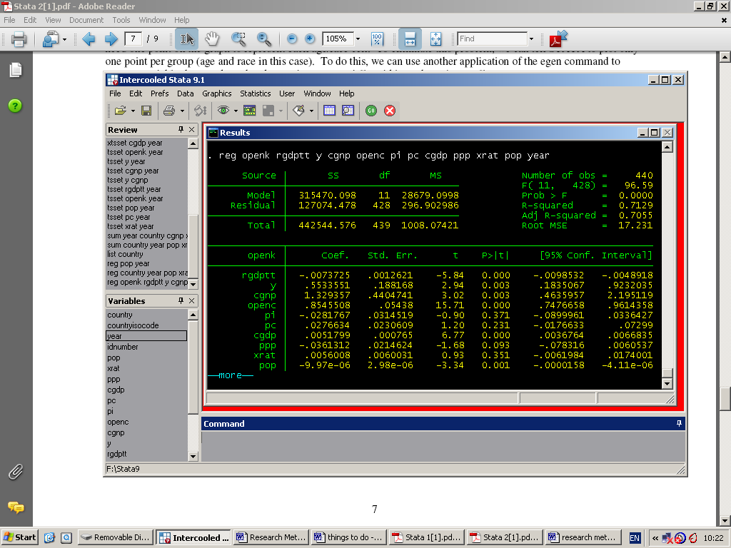
The first pass on the unedited data in Stata 9.0 (Figure 4 overleaf) revealed that openness of the economy (to foreign direct investments and trade) is a function of gap (the country’s GNP), OpenC (openness of consumption level or propensity for imported goods), and y (Income). We draw these conclusions from Stata output:

• The openness of the economy (expressed as % change in current prices) is predicted to increase by 1 (percent) for every change of 1.33 in CGDP, ceteris paribus. The associated t value is high enough at 3.02 that such a result could have occurred by chance just three times in a thousand data points or re-sampling attempts.
• The second “most important” predictor variable appears to be OpenC because Open K is predicted to rise by 1 percent for every change of 0.94 in OpenC. For the computed t value of 15.71, p < 0.001. By definition, however, we must suspect autocorrelation at work here.
• In respect of the third key variable, OpenK is predicted to increase by 1 for every change of 0.55 in y (income but based on terms of ‘I$ terms of trade in 2000 Constant Prices’). Given that p < 0.001, the relationship could hardly have occurred by random variation alone.

The data also reveals an inverse relationship between the openness of the economy and PPP (parity purchasing power). However, this is a risk borne by free trade, that continuously adverse terms of trade will hurt the value of the domestic currency.

Except for the finding that the data does not support convergence (and, by implication, puts exogenous models in poor light), none of this is particularly relevant to the research question originally asked: can empirical validation be obtained for either model of economic growth?

No variable in the Penn World database acts as a proxy for, or directly measures, innovation propelled by investments in human capital. At the same time, visual inspection of annual growth rates in real GDP (Figure 3 above) provides no basis for concluding that divergence is a ‘real world’ phenomenon.

It is disappointing that this should be so given the moderately long period of data available: forty-four years’ worth of data points for the eight selected countries.

Recall, however, that the exogenous model takes into account population growth rate (n), depreciation (d), capital per worker (k), output/income per worker (y), the size of the labor force (L), and saving rate (s). The availability of investment in the database (expressed as a percentage of GDP at current prices) lays open the possibility of testing the model:

Growth rate of real GDP per capita (Chain) = α + β₁ ci (investment share of GDP)

+ β₂ ki (investment share of RGDPI)

+ β₃ pop (population)+ ε

Running the Penn World data again, with the addition of the U.S.A. to heighten the contrast between that industrialized nation and a less-developed country like Bangladesh, we find:

1. Reasonably good correlations between the dependent variable real GDP per capita and the independent variables ci (0.331), ki (0.342), and POP (0.285).
2. The model result is
3. Real GDP per capita = -1.67 -0.04(ci) + 0.254 (ki) + 0.000002 (POP) + 2.37
4. The t and p values for both investment variables do not meet minimum hurdles for statistical significance.
5. Since the only t value that meets the minimum hurdle of p < 0.05 is that for population (expressed in the Penn World database in thousands), we find some validation for the labor pool facet of exogenous theory. To wit, the beta coefficient is interpreted as saying that, all other things equal, real GDP per capita is predicted to increase by 0.0002 for every increase of one thousand in the nation’s population.
6. While the confidence level associated with this relationship is good, one concedes that labor pool alone is not a very good predictor of per-capita GDP.
7. Moreover, the model explains just 13% of the variance in real GDP per capita.

The likely next step consists of lagging the dependent variable on the assumption that investment and population both have lagged effects on a nation’s economic growth.

Bibliography

1. Butzin, B. D. (1997) An empirical analysis of the convergence hypothesis across countries: New evidence. (Unpublished Dissertation: Florida Atlantic University).
2. Heston, A., Summers R. & Aten, B. (2006, September) Penn World Table Version 6.2, Center for International Comparisons of Production, Income and Prices at the University of Pennsylvania.
3. Romer, P. M. (1986, Oct.) Increasing returns and long-run growth. The Journal of Political Economy, 94 (5): pp. 1002-1037.
4. Solow, R. M. (1956) A contribution to the theory of economic growth. Quarterly Journal of Economics, 70 (1): pp. 65–94.

Footnotes

1. Aoki and Yoshikawa, 2007. Page 7.
2. Monteils, 2002. Page 2.